【免费书稿《现代统计学入门(第二版)》】《Introduction to Modern Statistics (2nd Ed)》https://openintro-ims2.netlify.app/
【线性代数的艺术可视化图释中文版】‘The-Art-of-Linear-Algebra - Graphic notes on Gilbert Strang’s “Linear Algebra for Everyone”’ Kefang Liu GitHub: github.com/kf-liu/The-Art-of-Linear-Algebra-zh-CN
互联网上有很多有关提示的材料,例如《30 prompts everyone has to know》之类的文章。这些文章主要集中在 ChatGPT Web 用户界面上,许多人在使用它执行特定的、通常是一次性的任务。但是,我认为 LLM 或大型语言模型作为开发人员的更强大功能是使用 API 调用到 LLM,以快速构建软件应用程序。我认为这方面还没有得到充分的重视。实际上,我们在 DeepLearning.AI 的姊妹公司 AI Fund 的团队一直在与许多初创公司合作,将这些技术应用于许多不同的应用程序上。看到 LLM API 能够让开发人员非常快速地构建应用程序,这真是令人兴奋。
当然,如果你想象一下让一位新毕业的大学生为你完成这个任务,你甚至可以提前指定他们应该阅读哪些文本片段来写关于 Alan Turing的文本,那么这能够帮助这位新毕业的大学生更好地成功完成这项任务。下一章你会看到如何让提示清晰明确,创建提示的一个重要原则,你还会从提示的第二个原则中学到给LLM时间去思考。
# 中文版见下一个 celltext=f"""
You should express what you want a model to do by \
providing instructions that are as clear and \
specific as you can possibly make them. \
This will guide the model towards the desired output, \
and reduce the chances of receiving irrelevant \
or incorrect responses. Don't confuse writing a \
clear prompt with writing a short prompt. \
In many cases, longer prompts provide more clarity \
and context for the model, which can lead to \
more detailed and relevant outputs.
"""prompt=f"""
Summarize the text delimited by triple backticks \
into a single sentence.
```{text}```
"""response=get_completion(prompt)print(response)
Clear and specific instructions should be provided to guide a model towards the desired output, and longer prompts can provide more clarity and context for the model, leading to more detailed and relevant outputs.
prompt=f"""
Generate a list of three made-up book titles along \
with their authors and genres.
Provide them in JSON format with the following keys:
book_id, title, author, genre.
"""response=get_completion(prompt)print(response)
[
{
"book_id": 1,
"title": "The Lost City of Zorath",
"author": "Aria Blackwood",
"genre": "Fantasy"
},
{
"book_id": 2,
"title": "The Last Survivors",
"author": "Ethan Stone",
"genre": "Science Fiction"
},
{
"book_id": 3,
"title": "The Secret Life of Bees",
"author": "Lila Rose",
"genre": "Romance"
}
]
text_1=f"""
Making a cup of tea is easy! First, you need to get some \
water boiling. While that's happening, \
grab a cup and put a tea bag in it. Once the water is \
hot enough, just pour it over the tea bag. \
Let it sit for a bit so the tea can steep. After a \
few minutes, take out the tea bag. If you \
like, you can add some sugar or milk to taste. \
And that's it! You've got yourself a delicious \
cup of tea to enjoy.
"""prompt=f"""
You will be provided with text delimited by triple quotes.
If it contains a sequence of instructions, \
re-write those instructions in the following format:
Step 1 - ...
Step 2 - …
…
Step N - …
If the text does not contain a sequence of instructions, \
then simply write \"No steps provided.\"\"\"\"{text_1}\"\"\""""response=get_completion(prompt)print("Completion for Text 1:")print(response)
Completion for Text 1:
Step 1 - Get some water boiling.
Step 2 - Grab a cup and put a tea bag in it.
Step 3 - Once the water is hot enough, pour it over the tea bag.
Step 4 - Let it sit for a bit so the tea can steep.
Step 5 - After a few minutes, take out the tea bag.
Step 6 - Add some sugar or milk to taste.
Step 7 - Enjoy your delicious cup of tea!
英语例子2
text_2=f"""
The sun is shining brightly today, and the birds are \
singing. It's a beautiful day to go for a \
walk in the park. The flowers are blooming, and the \
trees are swaying gently in the breeze. People \
are out and about, enjoying the lovely weather. \
Some are having picnics, while others are playing \
games or simply relaxing on the grass. It's a \
perfect day to spend time outdoors and appreciate the \
beauty of nature.
"""prompt=f"""You will be provided with text delimited by triple quotes.
If it contains a sequence of instructions, \
re-write those instructions in the following format:
Step 1 - ...
Step 2 - …
…
Step N - …
If the text does not contain a sequence of instructions, \
then simply write \"No steps provided.\"\"\"\"{text_2}\"\"\""""response=get_completion(prompt)print("Completion for Text 2:")print(response)
prompt=f"""
Your task is to answer in a consistent style.
<child>: Teach me about patience.
<grandparent>: The river that carves the deepest \
valley flows from a modest spring; the \
grandest symphony originates from a single note; \
the most intricate tapestry begins with a solitary thread.
<child>: Teach me about resilience.
"""response=get_completion(prompt)print(response)
<grandparent>: Resilience is like a tree that bends with the wind but never breaks. It is the ability to bounce back from adversity and keep moving forward, even when things get tough. Just like a tree that grows stronger with each storm it weathers, resilience is a quality that can be developed and strengthened over time.
text=f"""
In a charming village, siblings Jack and Jill set out on \
a quest to fetch water from a hilltop \
well. As they climbed, singing joyfully, misfortune \
struck—Jack tripped on a stone and tumbled \
down the hill, with Jill following suit. \
Though slightly battered, the pair returned home to \
comforting embraces. Despite the mishap, \
their adventurous spirits remained undimmed, and they \
continued exploring with delight.
"""# example 1prompt_1=f"""
Perform the following actions:
1 - Summarize the following text delimited by triple \
backticks with 1 sentence.
2 - Translate the summary into French.
3 - List each name in the French summary.
4 - Output a json object that contains the following \
keys: french_summary, num_names.
Separate your answers with line breaks.
Text:
```{text}```
"""response=get_completion(prompt_1)print("Completion for prompt 1:")print(response)
Completion for prompt 1:
Two siblings, Jack and Jill, go on a quest to fetch water from a well on a hilltop, but misfortune strikes and they both tumble down the hill, returning home slightly battered but with their adventurous spirits undimmed.
Deux frères et sœurs, Jack et Jill, partent en quête d'eau d'un puits sur une colline, mais un malheur frappe et ils tombent tous les deux de la colline, rentrant chez eux légèrement meurtris mais avec leurs esprits aventureux intacts.
Noms: Jack, Jill.
{
"french_summary": "Deux frères et sœurs, Jack et Jill, partent en quête d'eau d'un puits sur une colline, mais un malheur frappe et ils tombent tous les deux de la colline, rentrant chez eux légèrement meurtris mais avec leurs esprits aventureux intacts.",
"num_names": 2
}
prompt 1:
1-兄妹在山顶井里打水时发生意外,但仍然保持冒险精神。
2-Dans un charmant village, les frère et sœur Jack et Jill partent chercher de l'eau dans un puits au sommet de la montagne. Malheureusement, Jack trébuche sur une pierre et tombe de la montagne, suivi de près par Jill. Bien qu'ils soient légèrement blessés, ils retournent chez eux chaleureusement. Malgré cet accident, leur esprit d'aventure ne diminue pas et ils continuent à explorer joyeusement.
3-Jack, Jill
4-{
"French_summary": "Dans un charmant village, les frère et sœur Jack et Jill partent chercher de l'eau dans un puits au sommet de la montagne. Malheureusement, Jack trébuche sur une pierre et tombe de la montagne, suivi de près par Jill. Bien qu'ils soient légèrement blessés, ils retournent chez eux chaleureusement. Malgré cet accident, leur esprit d'aventure ne diminue pas et ils continuent à explorer joyeusement.",
"num_names": 2
}
英语例子2
prompt_2=f"""
Your task is to perform the following actions:
1 - Summarize the following text delimited by <> with 1 sentence.
2 - Translate the summary into French.
3 - List each name in the French summary.
4 - Output a json object that contains the
following keys: french_summary, num_names.
Use the following format:
Text: <text to summarize>
Summary: <summary>
Translation: <summary translation>
Names: <list of names in French summary>
Output JSON: <json with summary and num_names>
Text: <{text}>
"""response=get_completion(prompt_2)print("\nCompletion for prompt 2:")print(response)
Completion for prompt 2:
Summary: 兄妹杰克和吉尔在山顶井里打水时发生意外,但他们仍然保持冒险精神继续探索。
Translation: Jack and Jill, deux frères et sœurs, ont eu un accident en allant chercher de l'eau dans un puits de montagne, mais ils ont continué à explorer avec un esprit d'aventure.
Names: Jack, Jill
Output JSON: {"french_summary": "Jack and Jill, deux frères et sœurs, ont eu un accident en allant chercher de l'eau dans un puits de montagne, mais ils ont continué à explorer avec un esprit d'aventure.", "num_names": 2}
prompt 2:
摘要:兄妹杰克和吉尔在迷人的村庄里冒险,不幸摔伤后回到家中,但仍然充满冒险精神。
翻译:In a charming village, siblings Jack and Jill set out to fetch water from a mountaintop well. While climbing and singing, Jack trips on a stone and tumbles down the mountain, with Jill following closely behind. Despite some bruises, they make it back home safely. Their adventurous spirit remains undiminished as they continue to explore with joy.
名称:Jack,Jill
输出 JSON:{"English_summary": "In a charming village, siblings Jack and Jill set out to fetch water from a mountaintop well. While climbing and singing, Jack trips on a stone and tumbles down the mountain, with Jill following closely behind. Despite some bruises, they make it back home safely. Their adventurous spirit remains undiminished as they continue to explore with joy.", "num_names": 2}
策略二:指导模型在下结论之前找出一个自己的解法
有时候,在明确指导模型在做决策之前要思考解决方案时,我们会得到更好的结果。
接下来我们会给出一个问题和一个学生的解答,要求模型判断解答是否正确
英语例子1
prompt=f"""
Determine if the student's solution is correct or not.
Question:
I'm building a solar power installation and I need \
help working out the financials.
- Land costs $100 / square foot
- I can buy solar panels for $250 / square foot
- I negotiated a contract for maintenance that will cost \
me a flat $100k per year, and an additional $10 / square \
foot
What is the total cost for the first year of operations
as a function of the number of square feet.
Student's Solution:
Let x be the size of the installation in square feet.
Costs:
1. Land cost: 100x
2. Solar panel cost: 250x
3. Maintenance cost: 100,000 + 100x
学生的解决方案:
设x为发电站的大小,单位为平方英尺。
费用:
Total cost: 100x + 250x + 100,000 + 100x = 450x + 100,000
"""response=get_completion(prompt)print(response)
prompt=f"""
Your task is to determine if the student's solution \
is correct or not.
To solve the problem do the following:
- First, work out your own solution to the problem.
- Then compare your solution to the student's solution \
and evaluate if the student's solution is correct or not.
Don't decide if the student's solution is correct until
you have done the problem yourself.
Use the following format:
Question:
```
question here
```
Student's solution:
```
student's solution here
```
Actual solution:
```
steps to work out the solution and your solution here
```
Is the student's solution the same as actual solution \
just calculated:
```
yes or no
```
Student grade:
```
correct or incorrect
```
Question:
```
I'm building a solar power installation and I need help \
working out the financials.
- Land costs $100 / square foot
- I can buy solar panels for $250 / square foot
- I negotiated a contract for maintenance that will cost \
me a flat $100k per year, and an additional $10 / square \
foot
What is the total cost for the first year of operations \
as a function of the number of square feet.
```
Student's solution:
```
Let x be the size of the installation in square feet.
Costs:
1. Land cost: 100x
2. Solar panel cost: 250x
3. Maintenance cost: 100,000 + 100x
Total cost: 100x + 250x + 100,000 + 100x = 450x + 100,000
```
Actual solution:
"""response=get_completion(prompt)print(response)
Let x be the size of the installation in square feet.
Costs:
1. Land cost: 100x
2. Solar panel cost: 250x
3. Maintenance cost: 100,000 + 10x
Total cost: 100x + 250x + 100,000 + 10x = 360x + 100,000
Is the student's solution the same as actual solution just calculated:
No
Student grade:
Incorrect
prompt=f"""
Tell me about AeroGlide UltraSlim Smart Toothbrush by Boie
"""response=get_completion(prompt)print(response)
The AeroGlide UltraSlim Smart Toothbrush by Boie is a high-tech toothbrush that uses advanced sonic technology to provide a deep and thorough clean. It features a slim and sleek design that makes it easy to hold and maneuver, and it comes with a range of smart features that help you optimize your brushing routine.
One of the key features of the AeroGlide UltraSlim Smart Toothbrush is its advanced sonic technology, which uses high-frequency vibrations to break up plaque and bacteria on your teeth and gums. This technology is highly effective at removing even the toughest stains and buildup, leaving your teeth feeling clean and fresh.
In addition to its sonic technology, the AeroGlide UltraSlim Smart Toothbrush also comes with a range of smart features that help you optimize your brushing routine. These include a built-in timer that ensures you brush for the recommended two minutes, as well as a pressure sensor that alerts you if you're brushing too hard.
Overall, the AeroGlide UltraSlim Smart Toothbrush by Boie is a highly advanced and effective toothbrush that is perfect for anyone looking to take their oral hygiene to the next level. With its advanced sonic technology and smart features, it provides a deep and thorough clean that leaves your teeth feeling fresh and healthy.
# 示例:产品说明书fact_sheet_chair="""
OVERVIEW
- Part of a beautiful family of mid-century inspired office furniture,
including filing cabinets, desks, bookcases, meeting tables, and more.
- Several options of shell color and base finishes.
- Available with plastic back and front upholstery (SWC-100)
or full upholstery (SWC-110) in 10 fabric and 6 leather options.
- Base finish options are: stainless steel, matte black,
gloss white, or chrome.
- Chair is available with or without armrests.
- Suitable for home or business settings.
- Qualified for contract use.
CONSTRUCTION
- 5-wheel plastic coated aluminum base.
- Pneumatic chair adjust for easy raise/lower action.
DIMENSIONS
- WIDTH 53 CM | 20.87”
- DEPTH 51 CM | 20.08”
- HEIGHT 80 CM | 31.50”
- SEAT HEIGHT 44 CM | 17.32”
- SEAT DEPTH 41 CM | 16.14”
OPTIONS
- Soft or hard-floor caster options.
- Two choices of seat foam densities:
medium (1.8 lb/ft3) or high (2.8 lb/ft3)
- Armless or 8 position PU armrests
MATERIALS
SHELL BASE GLIDER
- Cast Aluminum with modified nylon PA6/PA66 coating.
- Shell thickness: 10 mm.
SEAT
- HD36 foam
COUNTRY OF ORIGIN
- Italy
"""
# 提示:基于说明书生成营销描述prompt=f"""
Your task is to help a marketing team create a
description for a retail website of a product based
on a technical fact sheet.
Write a product description based on the information
provided in the technical specifications delimited by
triple backticks.
Technical specifications: ```{fact_sheet_chair}```
"""response=get_completion(prompt)print(response)
Introducing our stunning mid-century inspired office chair, the perfect addition to any home or business setting. Part of a beautiful family of office furniture, including filing cabinets, desks, bookcases, meeting tables, and more, this chair is available in several options of shell color and base finishes to suit your style. Choose from plastic back and front upholstery (SWC-100) or full upholstery (SWC-110) in 10 fabric and 6 leather options.
The chair is constructed with a 5-wheel plastic coated aluminum base and features a pneumatic chair adjust for easy raise/lower action. It is available with or without armrests and is qualified for contract use. The base finish options are stainless steel, matte black, gloss white, or chrome.
Measuring at a width of 53 cm, depth of 51 cm, and height of 80 cm, with a seat height of 44 cm and seat depth of 41 cm, this chair is designed for ultimate comfort. You can also choose between soft or hard-floor caster options and two choices of seat foam densities: medium (1.8 lb/ft3) or high (2.8 lb/ft3). The armrests are available in either an armless or 8 position PU option.
The materials used in the construction of this chair are of the highest quality. The shell base glider is made of cast aluminum with modified nylon PA6/PA66 coating and has a shell thickness of 10 mm. The seat is made of HD36 foam, ensuring maximum comfort and durability.
This chair is made in Italy and is the perfect combination of style and functionality. Upgrade your workspace with our mid-century inspired office chair today!
# 优化后的 Prompt,要求生成描述不多于 50 词prompt=f"""
Your task is to help a marketing team create a
description for a retail website of a product based
on a technical fact sheet.
Write a product description based on the information
provided in the technical specifications delimited by
triple backticks.
Use at most 50 words.
Technical specifications: ```{fact_sheet_chair}```
"""response=get_completion(prompt)print(response)
Introducing our beautiful medieval-style office furniture collection, including filing cabinets, desks, bookcases, and conference tables. Choose from a variety of shell colors and base coatings, with optional plastic or fabric/leather decoration. The chair features a plastic-coated aluminum base with five wheels and pneumatic height adjustment. Perfect for home or commercial use. Made in Italy.
# 优化后的 Prompt,说明面向对象,应具有什么性质且侧重于什么方面prompt=f"""
Your task is to help a marketing team create a
description for a retail website of a product based
on a technical fact sheet.
Write a product description based on the information
provided in the technical specifications delimited by
triple backticks.
The description is intended for furniture retailers,
so should be technical in nature and focus on the
materials the product is constructed from.
Use at most 50 words.
Technical specifications: ```{fact_sheet_chair}```
"""response=get_completion(prompt)print(response)
Introducing our beautiful medieval-style office furniture collection, including file cabinets, desks, bookcases, and conference tables. Available in multiple shell colors and base coatings, with optional plastic or fabric/leather upholstery. Features a plastic-coated aluminum base with five wheels and pneumatic chair adjustment. Suitable for home or commercial use and made with high-quality materials, including cast aluminum with a modified nylon coating and HD36 foam. Made in Italy.
# 更进一步,要求在描述末尾包含 7个字符的产品IDprompt=f"""
Your task is to help a marketing team create a
description for a retail website of a product based
on a technical fact sheet.
Write a product description based on the information
provided in the technical specifications delimited by
triple backticks.
The description is intended for furniture retailers,
so should be technical in nature and focus on the
materials the product is constructed from.
At the end of the description, include every 7-character
Product ID in the technical specification.
Use at most 50 words.
Technical specifications: ```{fact_sheet_chair}```
"""response=get_completion(prompt)print(response)
Introducing our beautiful medieval-style office furniture collection, featuring file cabinets, desks, bookshelves, and conference tables. Available in multiple shell colors and base coatings, with optional plastic or fabric/leather decorations. The chair comes with or without armrests and has a plastic-coated aluminum base with five wheels and pneumatic height adjustment. Suitable for home or commercial use. Made in Italy.
Product IDs: SWC-100, SWC-110
# 要求它抽取信息并组织成表格,并指定表格的列、表名和格式prompt=f"""
Your task is to help a marketing team create a
description for a retail website of a product based
on a technical fact sheet.
Write a product description based on the information
provided in the technical specifications delimited by
triple backticks.
The description is intended for furniture retailers,
so should be technical in nature and focus on the
materials the product is constructed from.
At the end of the description, include every 7-character
Product ID in the technical specification.
After the description, include a table that gives the
product's dimensions. The table should have two columns.
In the first column include the name of the dimension.
In the second column include the measurements in inches only.
Give the table the title 'Product Dimensions'.
Format everything as HTML that can be used in a website.
Place the description in a <div> element.
Technical specifications: ```{fact_sheet_chair}```
"""response=get_completion(prompt)print(response)
<div>
<p>Introducing our beautiful collection of medieval-style office furniture, including file cabinets, desks, bookcases, and conference tables. Choose from a variety of shell colors and base coatings. You can opt for plastic front and backrest decoration (SWC-100) or full decoration with 10 fabrics and 6 leathers (SWC-110). Base coating options include stainless steel, matte black, glossy white, or chrome. The chair is available with or without armrests and is suitable for both home and commercial settings. It is contract eligible.</p>
<p>The structure features a plastic-coated aluminum base with five wheels. The chair is pneumatically adjustable for easy height adjustment.</p>
<p>Product IDs: SWC-100, SWC-110</p>
<table>
<caption>Product Dimensions</caption>
<tr>
<td>Width</td>
<td>20.87 inches</td>
</tr>
<tr>
<td>Depth</td>
<td>20.08 inches</td>
</tr>
<tr>
<td>Height</td>
<td>31.50 inches</td>
</tr>
<tr>
<td>Seat Height</td>
<td>17.32 inches</td>
</tr>
<tr>
<td>Seat Depth</td>
<td>16.14 inches</td>
</tr>
</table>
<p>Options include soft or hard floor casters. You can choose from two seat foam densities: medium (1.8 pounds/cubic foot) or high (2.8 pounds/cubic foot). The chair is available with or without 8-position PU armrests.</p>
<p>Materials:</p>
<ul>
<li>Shell, base, and sliding parts: cast aluminum coated with modified nylon PA6/PA66. Shell thickness: 10mm.</li>
<li>Seat: HD36 foam</li>
</ul>
<p>Made in Italy.</p>
</div>
# 表格是以 HTML 格式呈现的,加载出来fromIPython.displayimportdisplay,HTMLdisplay(HTML(response))
prod_review="""
Got this panda plush toy for my daughter's birthday, \
who loves it and takes it everywhere. It's soft and \
super cute, and its face has a friendly look. It's \
a bit small for what I paid though. I think there \
might be other options that are bigger for the \
same price. It arrived a day earlier than expected, \
so I got to play with it myself before I gave it \
to her.
"""
prompt=f"""
Your task is to generate a short summary of a product \
review from an ecommerce site.
Summarize the review below, delimited by triple
backticks, in at most 30 words.
Review: ```{prod_review}```
"""response=get_completion(prompt)print(response)
Soft and cute panda plush toy loved by daughter, but a bit small for the price. Arrived early.
prompt=f"""
Your task is to generate a short summary of a product \
review from an ecommerce site to give feedback to the \
Shipping deparmtment.
Summarize the review below, delimited by triple
backticks, in at most 30 words, and focusing on any aspects \
that mention shipping and delivery of the product.
Review: ```{prod_review}```
"""response=get_completion(prompt)print(response)
The panda plush toy arrived a day earlier than expected, but the customer felt it was a bit small for the price paid.
prompt=f"""
Your task is to generate a short summary of a product \
review from an ecommerce site to give feedback to the \
pricing deparmtment, responsible for determining the \
price of the product.
Summarize the review below, delimited by triple
backticks, in at most 30 words, and focusing on any aspects \
that are relevant to the price and perceived value.
Review: ```{prod_review}```
"""response=get_completion(prompt)print(response)
The panda plush toy is soft, cute, and loved by the recipient, but the price may be too high for its size compared to other options.
prompt=f"""
Your task is to extract relevant information from \
a product review from an ecommerce site to give \
feedback to the Shipping department.
From the review below, delimited by triple quotes \
extract the information relevant to shipping and \
delivery. Limit to 30 words.
Review: ```{prod_review}```
"""response=get_completion(prompt)print(response)
"The product arrived a day earlier than expected."
review_1=prod_review# review for a standing lampreview_2="""
Needed a nice lamp for my bedroom, and this one \
had additional storage and not too high of a price \
point. Got it fast - arrived in 2 days. The string \
to the lamp broke during the transit and the company \
happily sent over a new one. Came within a few days \
as well. It was easy to put together. Then I had a \
missing part, so I contacted their support and they \
very quickly got me the missing piece! Seems to me \
to be a great company that cares about their customers \
and products.
"""# review for an electric toothbrushreview_3="""
My dental hygienist recommended an electric toothbrush, \
which is why I got this. The battery life seems to be \
pretty impressive so far. After initial charging and \
leaving the charger plugged in for the first week to \
condition the battery, I've unplugged the charger and \
been using it for twice daily brushing for the last \
3 weeks all on the same charge. But the toothbrush head \
is too small. I’ve seen baby toothbrushes bigger than \
this one. I wish the head was bigger with different \
length bristles to get between teeth better because \
this one doesn’t. Overall if you can get this one \
around the $50 mark, it's a good deal. The manufactuer's \
replacements heads are pretty expensive, but you can \
get generic ones that're more reasonably priced. This \
toothbrush makes me feel like I've been to the dentist \
every day. My teeth feel sparkly clean!
"""# review for a blenderreview_4="""
So, they still had the 17 piece system on seasonal \
sale for around $49 in the month of November, about \
half off, but for some reason (call it price gouging) \
around the second week of December the prices all went \
up to about anywhere from between $70-$89 for the same \
system. And the 11 piece system went up around $10 or \
so in price also from the earlier sale price of $29. \
So it looks okay, but if you look at the base, the part \
where the blade locks into place doesn’t look as good \
as in previous editions from a few years ago, but I \
plan to be very gentle with it (example, I crush \
very hard items like beans, ice, rice, etc. in the \
blender first then pulverize them in the serving size \
I want in the blender then switch to the whipping \
blade for a finer flour, and use the cross cutting blade \
first when making smoothies, then use the flat blade \
if I need them finer/less pulpy). Special tip when making \
smoothies, finely cut and freeze the fruits and \
vegetables (if using spinach-lightly stew soften the \
spinach then freeze until ready for use-and if making \
sorbet, use a small to medium sized food processor) \
that you plan to use that way you can avoid adding so \
much ice if at all-when making your smoothie. \
After about a year, the motor was making a funny noise. \
I called customer service but the warranty expired \
already, so I had to buy another one. FYI: The overall \
quality has gone done in these types of products, so \
they are kind of counting on brand recognition and \
consumer loyalty to maintain sales. Got it in about \
two days.
"""reviews=[review_1,review_2,review_3,review_4]
foriinrange(len(reviews)):prompt=f"""
Your task is to generate a short summary of a product \
review from an ecommerce site.
Summarize the review below, delimited by triple \
backticks in at most 20 words.
Review: ```{reviews[i]}```
"""response=get_completion(prompt)print(i,response,"\n")
0 Soft and cute panda plush toy loved by daughter, but a bit small for the price. Arrived early.
1 Affordable lamp with storage, fast shipping, and excellent customer service. Easy to assemble and missing parts were quickly replaced.
2 Good battery life, small toothbrush head, but effective cleaning. Good deal if bought around $50.
3 The product was on sale for $49 in November, but the price increased to $70-$89 in December. The base doesn't look as good as previous editions, but the reviewer plans to be gentle with it. A special tip for making smoothies is to freeze the fruits and vegetables beforehand. The motor made a funny noise after a year, and the warranty had expired. Overall quality has decreased.
大型语言模型的一个非常好的特点是,对于许多这样的任务,你只需要编写一个prompt即可开始产生结果,而不需要进行大量的工作。这极大地加快了应用程序开发的速度。你还可以只使用一个模型和一个 API 来执行许多不同的任务,而不需要弄清楚如何训练和部署许多不同的模型。
商品评论文本
这是一盏台灯的评论。
英语例子
lamp_review="""
Needed a nice lamp for my bedroom, and this one had \
additional storage and not too high of a price point. \
Got it fast. The string to our lamp broke during the \
transit and the company happily sent over a new one. \
Came within a few days as well. It was easy to put \
together. I had a missing part, so I contacted their \
support and they very quickly got me the missing piece! \
Lumina seems to me to be a great company that cares \
about their customers and products!!
"""
prompt=f"""
What is the sentiment of the following product review,
which is delimited with triple backticks?
Review text: ```{lamp_review}```
"""response=get_completion(prompt)print(response)
prompt=f"""
What is the sentiment of the following product review,
which is delimited with triple backticks?
Give your answer as a single word, either "positive" \
or "negative".
Review text: ```{lamp_review}```
"""response=get_completion(prompt)print(response)
prompt=f"""
Identify a list of emotions that the writer of the \
following review is expressing. Include no more than \
five items in the list. Format your answer as a list of \
lower-case words separated by commas.
Review text: ```{lamp_review}```
"""response=get_completion(prompt)print(response)
prompt=f"""
Is the writer of the following review expressing anger?\
The review is delimited with triple backticks. \
Give your answer as either yes or no.
Review text: ```{lamp_review}```
"""response=get_completion(prompt)print(response)
user_messages=["La performance du système est plus lente que d'habitude.",# System performance is slower than normal "Mi monitor tiene píxeles que no se iluminan.",# My monitor has pixels that are not lighting"Il mio mouse non funziona",# My mouse is not working"Mój klawisz Ctrl jest zepsuty",# My keyboard has a broken control key"我的屏幕在闪烁"# My screen is flashing]forissueinuser_messages:prompt=f"告诉我以下文本是什么语种,直接输出语种,如法语,无需输出标点符号: ```{issue}```"lang=get_completion(prompt)print(f"原始消息 ({lang}): {issue}\n")prompt=f"""
将以下消息分别翻译成英文和中文,并写成
中文翻译:xxx
英文翻译:yyy
的格式:
```{issue}```
"""response=get_completion(prompt)print(response,"\n=========================================")
原始消息 (法语): La performance du système est plus lente que d'habitude.
中文翻译:系统性能比平时慢。
英文翻译:The system performance is slower than usual.
=========================================
原始消息 (西班牙语): Mi monitor tiene píxeles que no se iluminan.
中文翻译:我的显示器有一些像素点不亮。
英文翻译:My monitor has pixels that don't light up.
=========================================
原始消息 (意大利语): Il mio mouse non funziona
中文翻译:我的鼠标不工作了。
英文翻译:My mouse is not working.
=========================================
原始消息 (波兰语): Mój klawisz Ctrl jest zepsuty
中文翻译:我的Ctrl键坏了
英文翻译:My Ctrl key is broken.
=========================================
原始消息 (中文): 我的屏幕在闪烁
中文翻译:我的屏幕在闪烁。
英文翻译:My screen is flickering.
=========================================
text=["The girl with the black and white puppies have a ball.",# The girl has a ball."Yolanda has her notebook.",# ok"Its going to be a long day. Does the car need it’s oil changed?",# Homonyms"Their goes my freedom. There going to bring they’re suitcases.",# Homonyms"Your going to need you’re notebook.",# Homonyms"That medicine effects my ability to sleep. Have you heard of the butterfly affect?",# Homonyms"This phrase is to cherck chatGPT for spelling abilitty"# spelling]foriinrange(len(text)):prompt=f"""请校对并更正以下文本,注意纠正文本保持原始语种,无需输出原始文本。
如果您没有发现任何错误,请说“未发现错误”。
例如:
输入:I are happy.
输出:I am happy.
```{text[i]}```"""response=get_completion(prompt)print(i,response)
0 The girl with the black and white puppies has a ball.
1 未发现错误。
2 It's going to be a long day. Does the car need its oil changed?
3 Their goes my freedom. They're going to bring their suitcases.
4 输出:You're going to need your notebook.
5 That medicine affects my ability to sleep. Have you heard of the butterfly effect?
6 This phrase is to check chatGPT for spelling ability.
text=f"""
Got this for my daughter for her birthday cuz she keeps taking \
mine from my room. Yes, adults also like pandas too. She takes \
it everywhere with her, and it's super soft and cute. One of the \
ears is a bit lower than the other, and I don't think that was \
designed to be asymmetrical. It's a bit small for what I paid for it \
though. I think there might be other options that are bigger for \
the same price. It arrived a day earlier than expected, so I got \
to play with it myself before I gave it to my daughter.
"""prompt=f"校对并更正以下商品评论:```{text}```"response=get_completion(prompt)print(response)
I got this for my daughter's birthday because she keeps taking mine from my room. Yes, adults also like pandas too. She takes it everywhere with her, and it's super soft and cute. However, one of the ears is a bit lower than the other, and I don't think that was designed to be asymmetrical. It's also a bit smaller than I expected for the price. I think there might be other options that are bigger for the same price. On the bright side, it arrived a day earlier than expected, so I got to play with it myself before giving it to my daughter.
response="""
I got this for my daughter's birthday because she keeps taking mine from my room. Yes, adults also like pandas too. She takes it everywhere with her, and it's super soft and cute. However, one of the ears is a bit lower than the other, and I don't think that was designed to be asymmetrical. It's also a bit smaller than I expected for the price. I think there might be other options that are bigger for the same price. On the bright side, it arrived a day earlier than expected, so I got to play with it myself before giving it to my daughter.
"""
text=f"""
Got this for my daughter for her birthday cuz she keeps taking \
mine from my room. Yes, adults also like pandas too. She takes \
it everywhere with her, and it's super soft and cute. One of the \
ears is a bit lower than the other, and I don't think that was \
designed to be asymmetrical. It's a bit small for what I paid for it \
though. I think there might be other options that are bigger for \
the same price. It arrived a day earlier than expected, so I got \
to play with it myself before I gave it to my daughter.
"""
# given the sentiment from the lesson on "inferring",# and the original customer message, customize the emailsentiment="negative"# review for a blenderreview=f"""
So, they still had the 17 piece system on seasonal \
sale for around $49 in the month of November, about \
half off, but for some reason (call it price gouging) \
around the second week of December the prices all went \
up to about anywhere from between $70-$89 for the same \
system. And the 11 piece system went up around $10 or \
so in price also from the earlier sale price of $29. \
So it looks okay, but if you look at the base, the part \
where the blade locks into place doesn’t look as good \
as in previous editions from a few years ago, but I \
plan to be very gentle with it (example, I crush \
very hard items like beans, ice, rice, etc. in the \
blender first then pulverize them in the serving size \
I want in the blender then switch to the whipping \
blade for a finer flour, and use the cross cutting blade \
first when making smoothies, then use the flat blade \
if I need them finer/less pulpy). Special tip when making \
smoothies, finely cut and freeze the fruits and \
vegetables (if using spinach-lightly stew soften the \
spinach then freeze until ready for use-and if making \
sorbet, use a small to medium sized food processor) \
that you plan to use that way you can avoid adding so \
much ice if at all-when making your smoothie. \
After about a year, the motor was making a funny noise. \
I called customer service but the warranty expired \
already, so I had to buy another one. FYI: The overall \
quality has gone done in these types of products, so \
they are kind of counting on brand recognition and \
consumer loyalty to maintain sales. Got it in about \
two days.
"""
prompt=f"""
You are a customer service AI assistant.
Your task is to send an email reply to a valued customer.
Given the customer email delimited by ```, \
Generate a reply to thank the customer for their review.
If the sentiment is positive or neutral, thank them for \
their review.
If the sentiment is negative, apologize and suggest that \
they can reach out to customer service.
Make sure to use specific details from the review.
Write in a concise and professional tone.
Sign the email as `AI customer agent`.
Customer review: ```{review}```
Review sentiment: {sentiment}"""response=get_completion(prompt)print(response)
Dear Valued Customer,
Thank you for taking the time to leave a review about our product. We are sorry to hear that you experienced an increase in price and that the quality of the product did not meet your expectations. We apologize for any inconvenience this may have caused you.
We would like to assure you that we take all feedback seriously and we will be sure to pass your comments along to our team. If you have any further concerns, please do not hesitate to reach out to our customer service team for assistance.
Thank you again for your review and for choosing our product. We hope to have the opportunity to serve you better in the future.
Best regards,
AI customer agent
# given the sentiment from the lesson on "inferring",# and the original customer message, customize the emailsentiment="negative"# review for a blenderreview=f"""
So, they still had the 17 piece system on seasonal \
sale for around $49 in the month of November, about \
half off, but for some reason (call it price gouging) \
around the second week of December the prices all went \
up to about anywhere from between $70-$89 for the same \
system. And the 11 piece system went up around $10 or \
so in price also from the earlier sale price of $29. \
So it looks okay, but if you look at the base, the part \
where the blade locks into place doesn’t look as good \
as in previous editions from a few years ago, but I \
plan to be very gentle with it (example, I crush \
very hard items like beans, ice, rice, etc. in the \
blender first then pulverize them in the serving size \
I want in the blender then switch to the whipping \
blade for a finer flour, and use the cross cutting blade \
first when making smoothies, then use the flat blade \
if I need them finer/less pulpy). Special tip when making \
smoothies, finely cut and freeze the fruits and \
vegetables (if using spinach-lightly stew soften the \
spinach then freeze until ready for use-and if making \
sorbet, use a small to medium sized food processor) \
that you plan to use that way you can avoid adding so \
much ice if at all-when making your smoothie. \
After about a year, the motor was making a funny noise. \
I called customer service but the warranty expired \
already, so I had to buy another one. FYI: The overall \
quality has gone done in these types of products, so \
they are kind of counting on brand recognition and \
consumer loyalty to maintain sales. Got it in about \
two days.
"""
prompt=f"""
You are a customer service AI assistant.
Your task is to send an email reply to a valued customer.
Given the customer email delimited by ```, \
Generate a reply to thank the customer for their review.
If the sentiment is positive or neutral, thank them for \
their review.
If the sentiment is negative, apologize and suggest that \
they can reach out to customer service.
Make sure to use specific details from the review.
Write in a concise and professional tone.
Sign the email as `AI customer agent`.
Customer review: ```{review}```
Review sentiment: {sentiment}"""response=get_completion(prompt,temperature=0.7)print(response)
Dear valued customer,
Thank you for taking the time to share your review with us. We are sorry to hear that you were disappointed with the prices of our products and the quality of our blender. We apologize for any inconvenience this may have caused you.
We value your feedback and would like to make things right for you. Please feel free to contact our customer service team so we can assist you with any concerns or issues you may have. We are committed to providing you with the best possible service and products.
Thank you again for your review and for being a loyal customer. We hope to have the opportunity to serve you better in the future.
Sincerely,
AI customer agent
messages=[{'role':'system','content':'You are an assistant that speaks like Shakespeare.'},{'role':'user','content':'tell me a joke'},{'role':'assistant','content':'Why did the chicken cross the road'},{'role':'user','content':'I don\'t know'}]response=get_completion_from_messages(messages,temperature=1)print(response)
messages=[{'role':'system','content':'You are friendly chatbot.'},{'role':'user','content':'Hi, my name is Isa'}]response=get_completion_from_messages(messages,temperature=1)print(response)
Hello Isa! It's great to meet you. How can I assist you today?
messages=[{'role':'system','content':'You are friendly chatbot.'},{'role':'user','content':'Yes, can you remind me, What is my name?'}]response=get_completion_from_messages(messages,temperature=1)print(response)
I'm sorry, but since we don't have any personal information about you, I don't know your name. Can you please tell me your name?
messages=[{'role':'system','content':'You are friendly chatbot.'},{'role':'user','content':'Hi, my name is Isa'},{'role':'assistant','content':"Hi Isa! It's nice to meet you. \
Is there anything I can help you with today?"},{'role':'user','content':'Yes, you can remind me, What is my name?'}]response=get_completion_from_messages(messages,temperature=1)print(response)
importpanelaspn# GUIpn.extension()panels=[]# collect display context=[{'role':'system','content':"""
You are OrderBot, an automated service to collect orders for a pizza restaurant. \
You first greet the customer, then collects the order, \
and then asks if it's a pickup or delivery. \
You wait to collect the entire order, then summarize it and check for a final \
time if the customer wants to add anything else. \
If it's a delivery, you ask for an address. \
Finally you collect the payment.\
Make sure to clarify all options, extras and sizes to uniquely \
identify the item from the menu.\
You respond in a short, very conversational friendly style. \
The menu includes \
pepperoni pizza 12.95, 10.00, 7.00 \
cheese pizza 10.95, 9.25, 6.50 \
eggplant pizza 11.95, 9.75, 6.75 \
fries 4.50, 3.50 \
greek salad 7.25 \
Toppings: \
extra cheese 2.00, \
mushrooms 1.50 \
sausage 3.00 \
canadian bacon 3.50 \
AI sauce 1.50 \
peppers 1.00 \
Drinks: \
coke 3.00, 2.00, 1.00 \
sprite 3.00, 2.00, 1.00 \
bottled water 5.00 \
"""}]# accumulate messagesinp=pn.widgets.TextInput(value="Hi",placeholder='Enter text here…')button_conversation=pn.widgets.Button(name="Chat!")interactive_conversation=pn.bind(collect_messages,button_conversation)dashboard=pn.Column(inp,pn.Row(button_conversation),pn.panel(interactive_conversation,loading_indicator=True,height=300),)
messages=context.copy()messages.append({'role':'system','content':'create a json summary of the previous food order. Itemize the price for each item\
The fields should be 1) pizza, include size 2) list of toppings 3) list of drinks, include size 4) list of sides include size 5)total price '},)#The fields should be 1) pizza, price 2) list of toppings 3) list of drinks, include size include price 4) list of sides include size include price, 5)total price '}, response=get_completion_from_messages(messages,temperature=0)print(response)
$ cd ~/projects/<module>
$ git log # log shows commits from Project <module>$ cd ~/projects/<module>/<sub_dir>
$ git log # still commits from Project <module>$ cd ~/projects/<module>/<submodule>
$ git log # commits from <submodule>
remote: Support for password authentication was removed on August 13, 2021. Please use a personal access token instead.
remote: Please see https://github.blog/2020-12-15-token-authentication-requirements-for-git-operations/ for more information.
fatal: 无法访问 'https://github.com/iphysresearch/GWToolkit.git/':The requested URL returned error: 403
As previously announced, starting on August 13, 2021, at 09:00 PST, we will no longer accept account passwords when authenticating Git operations on GitHub.com. Instead, token-based authentication (for example, personal access, OAuth, SSH Key, or GitHub App installation token) will be required for all authenticated Git operations.
Please refer to this blog post for instructions on what you need to do to continue using git operations securely.
模型选择 (model selection) 是统计推断专题里一个很重要的话题,对于引力波数据处理,引力波天文学和多信使天文学来说,尤是如此。此文是于 2021.1.19 在 ITP-CAS 为 Journal Club 准备的一个整理与调研。算是自己对 model selection 在个人在当前理解程度上的一个记录。
Bayes Inference
A primary aim of modern Bayesian inference is to construct a posterior distribution
$$
p(\theta|d)
$$
where $\theta$ is the set of model parameters and $d$ is the data associated with a measurement1. The posterior distribution $p(\theta|d)$ is the probability density function for the continuous variable $\theta$ (i.e. 15 parameters describing a CBC) given the data $d$ (strain data from a network of GW detectors). The probability that the true value of $\theta$ is between $(\theta’,\theta’+d\theta)$ is given by $p(\theta’|d)d\theta’$. It is normalised so that
$$
\int d\theta p(\theta|d) = 1 .
$$
According to Bayes theorem, the posterior distribution for multimessenger astrophysics is given by
$$
p(\theta \mid d)=\frac{\mathcal{L}(d \mid \theta) \pi(\theta)}{\mathcal{Z}}
$$
where $\mathcal{L}(d \mid \theta)$ is the likelihood function of the data given the $\theta$, $\pi(\theta)$ is the prior distribution of $\theta$, and $\mathcal{Z}$ is a normalisation factor called the ‘evidence’:
$$
\mathcal{Z} \equiv \int d \theta \mathcal{L}(d \mid \theta) \pi(\theta) .
$$
The likelihood function is something that we choose. It is a description of the measurement. By writing down a likelihood, we implicitly introduce a noise model. For GW astronomy, we typically assume a Gaussian-noise likelihood function that looks something like this
$$
\mathcal{L}(d \mid \theta)=\frac{1}{\sqrt{2 \pi \sigma^{2}}} \exp \left(-\frac{1}{2} \frac{(d-\mu(\theta))^{2}}{\sigma^{2}}\right) ,
$$
where $\mu(\theta)$ is a template for the gravitational strain waveform given $\theta$ and $\sigma$ is the detector noise. Note the $\pi$ with no parantheses and no subscript is the mathematical constent, not a prior distribution. This likelihood function reflects our assumption that the noise in GW detctors is Gaussian. Note that the likelihood function is not normalised with respect the $\theta$ and so $\int d\theta\mathcal{L}(d|\theta)\neq1$.
In practical terms, the evidence is a single number. It usually does not mean anything by itself, but becomes useful when we compare one evidence with another evidence. Formally, the evidence is a likelihood function. Specifically, it is the completely marginalised likelihood function. It is therefore sometimes denoted $\mathcal{L}(d)$ with no $\theta$ dependence. However, we prefer to use $\mathcal{Z}$ to denote the fully marginalised likelihood function.
Bayes Factor
Recall from probability theory:
We wish to distinguish between two hypotheses: $\mathcal{H}_{1}, \mathcal{H}_{2}$.
Bayes’s theorm can be expressed in a form mare convenient for our pruposes by employing the completeness relationship. Using the completeness relation (note: $P\left(\mathcal{H}_{1}\right)+P\left(\mathcal{H}_{2}\right)=1$), we find that the probability that $\mathcal{H}_{1}$ is true given that $d$ is true is
$$
\begin{aligned}
P(\mathcal{H}_{1} \mid d) &=\frac{P(\mathcal{H}_{1}) P(d \mid \mathcal{H}_{1})}{P(d)}\\
&=\frac{P\left(\mathcal{H}_{1}\right) P\left(d \mid \mathcal{H}_{1}\right)}{P\left(d \mid \mathcal{H}_{1}\right) P\left(\mathcal{H}_{1}\right)+P\left(d \mid \mathcal{H}_{2}\right) P\left(\mathcal{H}_{2}\right)} \\
&=\frac{\mathcal{\Lambda}\left(\mathcal{H}_{1} \mid d\right)}{\mathcal{\Lambda}\left(\mathcal{H}_{1} \mid d\right)+P\left(\mathcal{H}_{2}\right) / P\left(\mathcal{H}_{1}\right)} \\
&=\frac{\mathcal{O}\left(\mathcal{H}_{1} \mid d\right)}{\mathcal{O}\left(\mathcal{H}_{1} \mid d\right)+1}
\end{aligned}
$$
where we have defined likelihood ratio $\mathcal{\Lambda}$ and odds ratio $\mathcal{O}$:
$$
\begin{aligned}
\mathcal{\Lambda}\left(\mathcal{H}_{1} \mid d\right) &:=\frac{P\left(d \mid \mathcal{H}_{1}\right)}{P\left(d \mid \mathcal{H}_{0}\right)} \\
\mathcal{O}\left(\mathcal{H}_{1} \mid d\right) &:=\frac{P\left(\mathcal{H}_{1}\right)}{P\left(\mathcal{H}_{0}\right)}
\mathcal{\Lambda}\left(\mathcal{H}_{1} \mid d\right) = \frac{P\left(\mathcal{H}_{1}\right)}{P\left(\mathcal{H}_{0}\right)}
\frac{P\left(d \mid \mathcal{H}_{1}\right)}{P\left(d \mid \mathcal{H}_{0}\right)}
\end{aligned}
$$
The ratio of the evidence for two different models is called the Bayes factor. For example, we can compare the evidence for a BBH waveform predicted by general relativity (model $M_A$ with parameters $\theta$ ) with a BBH waveform predicted by some other theory (model $M_B$ with parameters $\nu$):
$$
\begin{aligned}
\mathcal{Z}_{A}&=\int d \theta \mathcal{L}\left(d \mid \theta, M_{A}\right) \pi(\theta) ,\\
\mathcal{Z}_{B}&=\int d \nu \mathcal{L}\left(d \mid \nu, M_{B}\right) \pi(\nu) .
\end{aligned}
$$
The A/B Bayes factor is
$$
\mathrm{BF}_{B}^{A}=\frac{\mathcal{Z}_{A}}{\mathcal{Z}_{B}} .
$$
Note that the number of parameters in $\nu$ can be different from the number of parameters in $\theta$.
Formally, the correct metric to compare two models is not the Bayes factor, but rather the odds ratio. The odds ratio is the product of the Bayes factor with the prior odds $\pi_A/\pi_B$, which describes our likelihood of hypotheses $A$ and $B$:
$$
\mathcal{O}_{B}^{A} \equiv \frac{\mathcal{Z}_{A}}{\mathcal{Z}_{B}} \frac{\pi_{A}}{\pi_{B}} =\frac{\pi_{A}}{\pi_{B}} \mathrm{BF}_{B}^{A}
$$
In many practical applications, we set the prior odds ratio to unity, and so the odds ratio is the Bayes factor. This practice is sensible in many applications where our intuition tells us: until we do this measurement both hypotheses are equally likely.
There are some (fairly uncommon) examples where we might choose a different prior odds ratio. For example, we may construct a model in which general relativity (GR) is wrong. We may further suppose that there are multiple different ways in which it could be wrong, each corresponding to a different GR-is-wrong sub-hypothesis. If we calculated the odds ratio comparing one of these GR-is-wrong sub-hypotheses to the GR-is-right hypothesis, we would not assign equal prior odds to both hypotheses. Rather, we would assign at most 50% probability to the entire GR-is-wrong hypothesis, which would then have to be split among the various sub-hypotheses.
Model Selection
Bayesian evidence encodes two pieces of information:
The likelihood tells us how well our model fits the data.
The act of marginalisation tell us about the size of the volume of parameter space we used to carry out a fit.
This creates a sort of tension:
We want to get the best fit possible (high likelihood) but with a minimum prior volume.
A model with a decent fit and a small prior volume often yields a greater evidence than a model with an excellent fit and a huge prior volume.
In these cases, the Bayes factor penalises the more complicated model for being too complicated.
How to understand this comments?
We can obtain some insights into the model evidence by making a simple approximation to the integral over parameters:
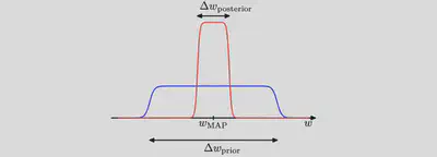
Consider first the case of a model having a single parameter $w$. ($N=1$)
Assume that the posterior distribution is sharply peaked around the most probable value $w_\text{MAP}$, with width $\Delta w_\text{posterior}$, then we can approximate the in- tegral by the value of the integrand at its maximum times the width of the peak.
Assume that the prior is flat with width $\Delta w_\text{prior}$ so that $\pi(w) = 1/\Delta w_\text{prior}$.
A rough approximation to the model evidence if we assume that the posterior distribution over parameters is sharply peaked around its mode $w_\text{MAP}$ .
then we have
$$
\mathcal{Z} \equiv \int d w \mathcal{L}(d \mid w) \pi(w) \simeq \mathcal{L}\left(\mathcal{d} \mid w_{\mathrm{MAP}}\right) \frac{\Delta w_{\text {posterior }}}{\Delta w_{\text {prior }}}
$$
and so taking logs we obtain (for a model having a set of $N$ parameters)
$$
\ln \mathcal{Z}(\mathcal{d}) \simeq \ln \mathcal{L}\left(\mathcal{d} \mid w_{\mathrm{MAP}}\right)+N\ln \left(\frac{\Delta w_{\text {posterior }}}{\Delta w_{\text {prior }}}\right)
$$
The first term: the fit to the data given by the most probable parameter values, and for a flat prior this would correspond to the log likelihood.
The second term (also called Occam factor) penalizes the model according to its complexity. Because $\Delta w_\text{posterior}<\Delta w_\text{prior}$ this term is negative, and it increases in magnitude as the ratio $\Delta w_\text{posterior}/\Delta w_\text{prior}$ gets smaller. Thus, if parameters are finely tuned to the data in the posterior distribution, then the penalty term is large.
Thus, in this very simple approximation, the size of the complexity penalty increases linearly with the number $N$ of adaptive parameters in the model. As we increase the complexity of the model, the first term will typically decrease, because a more complex model is better able to fit the data, whereas the second term will increase due to the dependence on $N$. The optimal model complexity, as determined by the maximum evidence, will be given by a trade-off between these two competing terms. We shall later develop a more refined version of this approximation, based on a Gaussian approximation to the posterior distribution.
A further insight into Bayesian model comparison and understand how the marginal likelihood can favour models of intermediate complexity by considering the Figure below.
Schematic illustration of the distribution of data sets for three models of different complexity, in which $M_1$ is the simplest and $M_3$ is the most complex. Note that the distributions are normalized. In this example, for the particular observed data set $\mathcal{D}_0$, the model $M_2$ with intermediate complexity has the largest evidence (the area und curve) .
Here the horizontal axis is a one-dimensional representation of the space of possible data sets, so that each point on this axis corresponds to a specific data set. We now consider three models $M_1$, $M_2$ and $M_3$ of successively increasing complexity. Imagine running these models generatively to produce example data sets, and then looking at the distribution of data sets that result. Any given model can generate a variety of different data sets since the parameters are governed by a prior probability distribution, and for any choice of the parameters there may be random noise on the target variables. To generate a particular data set from a specific model, we first choose the values of the parameters from their prior distribution $\pi(w)$, and then for these parameter values we sample the data from $\mathcal{L}(\mathcal{D}|w)$. Because the distributions $\mathcal{L}(\mathcal{D}|M_i)$ are normalized, we see that the particular data set $D_0$ can have the highest value of the evidence for the model of intermediate complexity. Essentially, the simpler model cannot fit the data well, whereas the more complex model spreads its predictive probability over too broad a range of data sets and so assigns relatively small probability to any one of them.
More insights:
If we compare two models where one model is a superset of the other—for example, we might compare GR and GR with non-tensor modes—and if the data are better explained by the simpler model, the log Bayes factor is typically modest,
$$
|\log \mathrm{BF}| \approx (1,2).
$$
Thus, it is difficult to completely rule out extensions to existing theories. We just obtain ever tighter constraints on the extended parameter space.
To make good use of Bayesian model comparison, we fully specify priors that are independent of the current data $\mathcal{D}$.
The sensitivity of the marginal likelihood to the prior range depends on the shape of the prior and is much greater for a uniform prior than a scale-invariant prior (see e.g. Gregory, 2005b, 61).
In most instances we are not particularly interested in the Occam factor itself, but only in the relative probabilities of the competing models as expressed by the Bayes factors. Because the Occam factor arises automatically in the marginalisation procedure, its effects will be present in any model-comparison calculation.
No Occam factors arise in parameter-estimation problems. Parameter estimation can be viewed as model comparison where the competing models have the same complexity so the Occam penalties are identical and cancel out.
On average the Bayes factor will always favour the correct model.
To see this, consider two models $\mathcal{M}_\text{true}$ and $\mathcal{M}_1$ in which the truth corresponds to $\mathcal{M}_\text{true}$. We assume that the true posterior distribution from which the data are considered is contained within the set of models under consideration. For a given finite data, it is possible for the Bayes factor to be larger for the incorrect model. However, if we average the Bayes factor over the distribution of data sets, we obtain the expected Bayes factor in the form
$$
\int \mathcal{Z}\left(\mathcal{D} \mid \mathcal{M}_{true}\right) \ln \frac{\mathcal{Z}\left(\mathcal{D} \mid \mathcal{M}_{true}\right)}{\mathcal{Z}\left(\mathcal{D} \mid \mathcal{M}_{1}\right)} \mathrm{d} \mathcal{D}
$$
where the average has been taken with respect to the true distribution of the data. This is an example of Kullback-Leibler divergence and satisfies the property of always being positive unless the two distributions are equal in which case it is zero. Thus on average the Bayes factor will always favour the correct model.
We have seen from Figure 1 that the model evidence can be sensitive to many aspects of the prior, such as the behaviour in the tails. Indeed, the evidence is not defined if the prior is improper, as can be seen by noting that an improper prior has an arbitrary scaling factor (in other words, the normalization coefficient is not defined because the distribution cannot be normalized). If we consider a proper prior and then take a suitable limit in order to obtain an improper prior (for example, a Gaussian prior in which we take the limit of infinite variance) then the evidence will go to zero, as can be seen Figure 1 and the equation below the Figure 1. It may, however, be possible to consider the evidence ratio between two models first and then take a limit to obtain a meaningful answer.
In a practical application, therefore, it will be wise to keep aside an independent test set of data on which to evaluate the overall performance of the final system.
By referring to model parameters, we are implicitly acknowledging that we begin with some model. Some authors make this explicit by writing the posterior as $p(\theta|d, M)$, where $M$ is the model. (Other authors sometimes use $I$ to denote the model.) We find this notation clunky and unnecessary since it goes without saying that one must always assume some model. If/when we consider two distinct models, we add an additional variable to denote the model. ↩︎
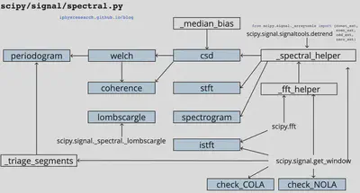
SciPy (pronounced “Sigh Pie”) is open-source software for mathematics, science, and engineering. It includes modules for statistics, optimization, integration, linear algebra, Fourier transforms, signal and image processing, ODE solvers, and more.
# Preparingmode='stft'# or psdsame_data=Trueoutdtype=np.result_type(x,np.complex64)# 明确数据精度axis=-1window='hann'boundary='zeros'padded=True# not useddetrend=False# not usedscaling='spectrum'# or densityreturn_onesided,sides=True,'onesided'fromscipy.signal._arraytoolsimportconst_ext,even_ext,odd_ext,zero_extboundary_funcs={'even':even_ext,'odd':odd_ext,'constant':const_ext,'zeros':zero_ext,None:None}
boundary_funcs 是考虑对数据 x 将会以什么样的形式来延拓其边界。后面很快会再讨论到这一点。
Finetune
下面的参数是比较重要的可调参数:
## Finetune ## # parse window; nperseg = win.shapenperseg=nperseg=fs//4nperseg=int(nperseg)print('nperseg = {}'.format(nperseg))# parse window; if array like, then set nperseg = win.shapewin,nperseg=signal.spectral._triage_segments(window,nperseg,input_length=x.shape[-1])print('nperseg = {}, win.size = {}'.format(nperseg,win.size))# win have the same dtype with outdtypeifnp.result_type(win,np.complex64)!=outdtype:win=win.astype(outdtype)# nfft must be greater than or equal to nperseg.nfft=int(fs//4)print('nfft = {}'.format(nfft))# noverlap must be less than nperseg.noverlap=int(fs//8)print('noverlap = {}'.format(noverlap))nstep=nperseg-noverlapprint('nstep = {}'.format(nstep))## output ### nperseg = 4096# nperseg = 4096, win.size = 4096# nfft = 4096# noverlap = 2048# nstep = 2048
nperseg 表示的是要解析的短时窗口序列的长度 (number of per segment)。
正式计算之前,还需要对我们的完整数据 x 进行边界延拓和补零的操作。下面的注释中也给出了这样操作偶的理由。
# Padding occurs after boundary extension, so that the extended signal ends# in zeros, instead of introducing an impulse at the end.# I.e. if x = [..., 3, 2]# extend then pad -> [..., 3, 2, 2, 3, 0, 0, 0]# pad then extend -> [..., 3, 2, 0, 0, 0, 2, 3]print('x.size = {}'.format(x.size))# boundary extensionx=boundary_funcs[boundary](x,nperseg//2,axis=-1)print('x.size = {} | {}'.format(x.size,hp.size+nperseg))# Pad to integer number of windowed segments# I.e make x.shape[-1] = nperseg + (nseg-1)*nstep, with integer nsegnadd=(-(x.shape[-1]-nperseg)%nstep)%npersegzeros_shape=list(x.shape[:-1])+[nadd]x=np.concatenate((x,np.zeros(zeros_shape)),axis=-1)print('x.size = {} | {}'.format(x.size,x.size%nperseg))## output ### x.size = 32613# x.size = 36709 | 36709# x.size = 36864 | 0
# Perform the windowed FFTsresult=_fft_helper(x,win,detrend_func,nperseg,noverlap,nfft,sides)def_fft_helper(x,win,detrend_func,nperseg,noverlap,nfft,sides):pass# ... (暂略)returnresult
Scipy 中原代码的实现其实非常 pythonic 风格的方法,那就是将数据 x 映射为一个数据矩阵,每行为每一个待处理的数据 segment,每列都是相同的 nperseg。
Way 1
# Created strided array of data segmentsifnperseg==1andnoverlap==0:result=x[...,np.newaxis]else:# https://stackoverflow.com/a/5568169step=nperseg-noverlapshape=x.shape[:-1]+((x.shape[-1]-noverlap)//step,nperseg)strides=x.strides[:-1]+(step*x.strides[-1],x.strides[-1])result=np.lib.stride_tricks.as_strided(x,shape=shape,strides=strides)
density: Select Power the loss of power is compensated. The ratio of the sum of the squared data before and after applying the window is used as a normalization factor. The total power within the spectrum therefore always corresponds to the power of the data before applying the window.
spectrum: Selecting Amplitude normalizes to the gain of the used window function, i.e. the sum of all values is divided by their number. This compensates the damping of the amplitudes caused by applying the window. This is especially useful to measure peaks within the spectrum.
ifsides=='onesided'andmode=='psd':# not used for stftifnfft%2:result[...,1:]*=2else:# Last point is unpaired Nyquist freq point, don't doubleresult[...,1:-1]*=2# All imaginary parts are zero anywaysifsame_dataandmode!='stft':result=result.real
>>>fromscipyimportsignal>>>importmatplotlib.pyplotasplt# Generate two test signals with some common features.>>>fs=10e3>>>N=1e5>>>amp=20>>>freq=1234.0>>>noise_power=0.001*fs/2>>>time=np.arange(N)/fs>>>b,a=signal.butter(2,0.25,'low')>>>x=np.random.normal(scale=np.sqrt(noise_power),size=time.shape)>>>y=signal.lfilter(b,a,x)>>>x+=amp*np.sin(2*np.pi*freq*time)>>>y+=np.random.normal(scale=0.1*np.sqrt(noise_power),size=time.shape)# Compute and plot the magnitude of the cross spectral density.>>>f,Pxy=signal.csd(x,y,fs,nperseg=1024)>>>f,Pxx=signal.csd(x,x,fs,nperseg=1024)>>>f,Pyy=signal.csd(y,y,fs,nperseg=1024)>>>plt.semilogy(f,np.abs(Pxy),label='Pxy')>>>plt.semilogy(f,np.abs(Pxx),label='Pxx')>>>plt.semilogy(f,np.abs(Pyy),label='Pyy')>>>plt.xlabel('frequency [Hz]')>>>plt.ylabel('CSD [V**2/Hz]')>>>plt.legend()>>>plt.show()
其源码的实现:
defcsd(x,y,fs=1.0,window='hann',nperseg=None,noverlap=None,nfft=None,detrend='constant',return_onesided=True,scaling='density',axis=-1,average='mean'):"""Estimate the cross power spectral density, Pxy, using Welch's method."""freqs,_,Pxy=_spectral_helper(x,y,fs,window,nperseg,noverlap,nfft,detrend,return_onesided,scaling,axis,mode='psd')# Average over windows.iflen(Pxy.shape)>=2andPxy.size>0:ifPxy.shape[-1]>1:ifaverage=='median':Pxy=np.median(Pxy,axis=-1)/_median_bias(Pxy.shape[-1])elifaverage=='mean':Pxy=Pxy.mean(axis=-1)else:raiseValueError('average must be "median" or "mean", got %s'%(average,))else:Pxy=np.reshape(Pxy,Pxy.shape[:-1])returnfreqs,Pxy
_median_bias
def_median_bias(n):"""
Returns the bias of the median of a set of periodograms relative to
the mean.
"""ii_2=2*np.arange(1.,(n-1)//2+1)return1+np.sum(1./(ii_2+1)-1./ii_2)
welch (PSD)
Estimate power spectral density using Welch’s method.
Welch’s method 1 computes an estimate of the power spectral density (PSD) by dividing the data into overlapping segments, computing a modified periodogram for each segment and averaging the periodograms.
源码是很简单直接的:
defwelch(x,fs=1.0,window='hann',nperseg=None,noverlap=None,nfft=None,detrend='constant',return_onesided=True,scaling='density',axis=-1,average='mean'):"""Estimate power spectral density using Welch's method."""freqs,Pxx=csd(x,x,fs=fs,window=window,nperseg=nperseg,noverlap=noverlap,nfft=nfft,detrend=detrend,return_onesided=return_onesided,scaling=scaling,axis=axis,average=average)returnfreqs,Pxx.real
这就是所谓的 Welch 方法下的 PSD。看个例子,体会一般:
>>>fromscipyimportsignal>>>importmatplotlib.pyplotasplt>>>np.random.seed(1234)# Generate a test signal, a 2 Vrms sine wave at 1234 Hz, corrupted by# 0.001 V**2/Hz of white noise sampled at 10 kHz.>>>fs=10e3>>>N=1e5>>>amp=2*np.sqrt(2)>>>freq=1234.0>>>noise_power=0.001*fs/2>>>time=np.arange(N)/fs>>>x=amp*np.sin(2*np.pi*freq*time)>>>x+=np.random.normal(scale=np.sqrt(noise_power),size=time.shape)
现在来计算并看看这个数据的 PSD,以及噪声的功率密度:
# Compute and plot the power spectral density.>>>f,Pxx_den=signal.welch(x,fs,nperseg=1024)>>>plt.semilogy(f,Pxx_den)>>>plt.ylim([0.5e-3,1])>>>plt.xlabel('frequency [Hz]')>>>plt.ylabel('PSD [V**2/Hz]')>>>plt.show()# If we average the last half of the spectral density, to exclude the# peak, we can recover the noise power on the signal.>>>np.mean(Pxx_den[256:])# 0.0009924865443739191
# Now compute and plot the power spectrum.>>>f,Pxx_spec=signal.welch(x,fs,'flattop',1024,scaling='spectrum')>>>plt.figure()>>>plt.semilogy(f,np.sqrt(Pxx_spec))>>>plt.xlabel('frequency [Hz]')>>>plt.ylabel('Linear spectrum [V RMS]')>>>plt.show()# The peak height in the power spectrum is an estimate of the RMS# amplitude.>>>np.sqrt(Pxx_spec.max())# 2.0077340678640727
# If we now introduce a discontinuity in the signal, by increasing the# amplitude of a small portion of the signal by 50, we can see the# corruption of the mean average power spectral density, but using a# median average better estimates the normal behaviour.>>>x[int(N//2):int(N//2)+10]*=50.>>>f,Pxx_den=signal.welch(x,fs,nperseg=1024)>>>f_med,Pxx_den_med=signal.welch(x,fs,nperseg=1024,average='median')>>>plt.semilogy(f,Pxx_den,label='mean')>>>plt.semilogy(f_med,Pxx_den_med,label='median')>>>plt.ylim([0.5e-3,1])>>>plt.xlabel('frequency [Hz]')>>>plt.ylabel('PSD [V**2/Hz]')>>>plt.legend()>>>plt.show()
coherence
Estimate the magnitude squared coherence estimate, Cxy, of discrete-time signals X and Y using Welch’s method.
Cxy = abs(Pxy)**2/(Pxx*Pyy), where Pxx and Pyy are power spectral density estimates of X and Y, and Pxy is the cross spectral density estimate of X and Y.
源码:
defcoherence(x,y,fs=1.0,window='hann',nperseg=None,noverlap=None,nfft=None,detrend='constant',axis=-1):"""
Estimate the magnitude squared coherence estimate, Cxy, of
discrete-time signals X and Y using Welch's method.
"""freqs,Pxx=welch(x,fs=fs,window=window,nperseg=nperseg,noverlap=noverlap,nfft=nfft,detrend=detrend,axis=axis)_,Pyy=welch(y,fs=fs,window=window,nperseg=nperseg,noverlap=noverlap,nfft=nfft,detrend=detrend,axis=axis)_,Pxy=csd(x,y,fs=fs,window=window,nperseg=nperseg,noverlap=noverlap,nfft=nfft,detrend=detrend,axis=axis)Cxy=np.abs(Pxy)**2/Pxx/Pyyreturnfreqs,Cxy
例子:
>>>fromscipyimportsignal>>>importmatplotlib.pyplotasplt# Generate two test signals with some common features.>>>fs=10e3>>>N=1e5>>>amp=20>>>freq=1234.0>>>noise_power=0.001*fs/2>>>time=np.arange(N)/fs>>>b,a=signal.butter(2,0.25,'low')>>>x=np.random.normal(scale=np.sqrt(noise_power),size=time.shape)>>>y=signal.lfilter(b,a,x)>>>x+=amp*np.sin(2*np.pi*freq*time)>>>y+=np.random.normal(scale=0.1*np.sqrt(noise_power),size=time.shape)# Compute and plot the coherence.>>>f,Cxy=signal.coherence(x,y,fs,nperseg=1024)>>>f,Pxx=signal.welch(x,fs,nperseg=1024)>>>f,Pyy=signal.welch(y,fs,nperseg=1024)>>>lnxy=plt.semilogy(f,Cxy,color='r',label='Cxy')>>>plt.ylabel('Coherence')>>>plt.twinx()>>>lnx=plt.semilogy(f,Pxx,color='g',label='Pxx')>>>lny=plt.semilogy(f,Pyy,color='b',label='Pyy')>>>plt.ylabel('PSD [V**2/Hz]')>>>plt.xlabel('frequency [Hz]')>>>lns=lnxy+lnx+lny>>>labs=[l.get_label()forlinlns]>>>plt.legend(lns,labs)>>>plt.show()
periodogram (PSD)
Estimate power spectral density using a periodogram.
下面是用 periodogram 计算 PSD 的源码:
defperiodogram(x,fs=1.0,window='boxcar',nfft=None,detrend='constant',return_onesided=True,scaling='density',axis=-1):"""Estimate power spectral density using a periodogram."""x=np.asarray(x)ifx.size==0:returnnp.empty(x.shape),np.empty(x.shape)ifwindowisNone:window='boxcar'ifnfftisNone:nperseg=x.shape[axis]elifnfft==x.shape[axis]:nperseg=nfftelifnfft>x.shape[axis]:nperseg=x.shape[axis]elifnfft<x.shape[axis]:s=[np.s_[:]]*len(x.shape)s[axis]=np.s_[:nfft]x=x[tuple(s)]nperseg=nfftnfft=Nonereturnwelch(x,fs=fs,window=window,nperseg=nperseg,noverlap=0,nfft=nfft,detrend=detrend,return_onesided=return_onesided,scaling=scaling,axis=axis)
例子:
>>>fromscipyimportsignal>>>importmatplotlib.pyplotasplt>>>np.random.seed(1234)# Generate a test signal, a 2 Vrms sine wave at 1234 Hz, corrupted by# 0.001 V**2/Hz of white noise sampled at 10 kHz.>>>fs=10e3>>>N=1e5>>>amp=2*np.sqrt(2)>>>freq=1234.0>>>noise_power=0.001*fs/2>>>time=np.arange(N)/fs>>>x=amp*np.sin(2*np.pi*freq*time)>>>x+=np.random.normal(scale=np.sqrt(noise_power),size=time.shape)# Compute and plot the power spectral density.>>>f,Pxx_den=signal.periodogram(x,fs)>>>plt.semilogy(f,Pxx_den)>>>plt.ylim([1e-7,1e2])>>>plt.xlabel('frequency [Hz]')>>>plt.ylabel('PSD [V**2/Hz]')>>>plt.show()# If we average the last half of the spectral density, to exclude the# peak, we can recover the noise power on the signal.>>>np.mean(Pxx_den[25000:])# 0.00099728892368242854
# Now compute and plot the power spectrum.>>>f,Pxx_spec=signal.periodogram(x,fs,'flattop',scaling='spectrum')>>>plt.figure()>>>plt.semilogy(f,np.sqrt(Pxx_spec))>>>plt.ylim([1e-4,1e1])>>>plt.xlabel('frequency [Hz]')>>>plt.ylabel('Linear spectrum [V RMS]')>>>plt.show()# The peak height in the power spectrum is an estimate of the RMS# amplitude.>>>np.sqrt(Pxx_spec.max())# 2.0077340678640727
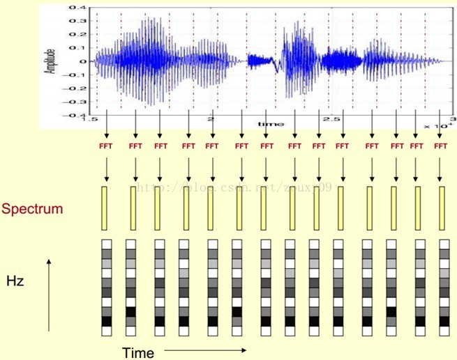
spectrogram
Compute a spectrogram with consecutive Fourier transforms.
Spectrograms can be used as a way of visualizing the change of a nonstationary signal’s frequency content over time.
源码:
defspectrogram(x,fs=1.0,window=('tukey',.25),nperseg=None,noverlap=None,nfft=None,detrend='constant',return_onesided=True,scaling='density',axis=-1,mode='psd'):"""Compute a spectrogram with consecutive Fourier transforms."""modelist=['psd','complex','magnitude','angle','phase']ifmodenotinmodelist:raiseValueError('unknown value for mode {}, must be one of {}'.format(mode,modelist))# need to set default for nperseg before setting default for noverlap belowwindow,nperseg=_triage_segments(window,nperseg,input_length=x.shape[axis])# Less overlap than welch, so samples are more statisically independentifnoverlapisNone:noverlap=nperseg//8ifmode=='psd':freqs,time,Sxx=_spectral_helper(x,x,fs,window,nperseg,noverlap,nfft,detrend,return_onesided,scaling,axis,mode='psd')else:freqs,time,Sxx=_spectral_helper(x,x,fs,window,nperseg,noverlap,nfft,detrend,return_onesided,scaling,axis,mode='stft')ifmode=='magnitude':Sxx=np.abs(Sxx)elifmodein['angle','phase']:Sxx=np.angle(Sxx)ifmode=='phase':# Sxx has one additional dimension for time stridesifaxis<0:axis-=1Sxx=np.unwrap(Sxx,axis=axis)# mode =='complex' is same as `stft`, doesn't need modificationreturnfreqs,time,Sxx
例子:
>>>fromscipyimportsignal>>>fromscipy.fftimportfftshift>>>importmatplotlib.pyplotasplt# Generate a test signal, a 2 Vrms sine wave whose frequency is slowly# modulated around 3kHz, corrupted by white noise of exponentially# decreasing magnitude sampled at 10 kHz.>>>fs=10e3>>>N=1e5>>>amp=2*np.sqrt(2)>>>noise_power=0.01*fs/2>>>time=np.arange(N)/float(fs)>>>mod=500*np.cos(2*np.pi*0.25*time)>>>carrier=amp*np.sin(2*np.pi*3e3*time+mod)>>>noise=np.random.normal(scale=np.sqrt(noise_power),size=time.shape)>>>noise*=np.exp(-time/5)>>>x=carrier+noise# Compute and plot the spectrogram.>>>f,t,Sxx=signal.spectrogram(x,fs)>>>plt.pcolormesh(t,f,Sxx,shading='gouraud')>>>plt.ylabel('Frequency [Hz]')>>>plt.xlabel('Time [sec]')>>>plt.show()
# Note, if using output that is not one sided, then use the following:>>>f,t,Sxx=signal.spectrogram(x,fs,return_onesided=False)>>>plt.pcolormesh(t,fftshift(f),fftshift(Sxx,axes=0),shading='gouraud')>>>plt.ylabel('Frequency [Hz]')>>>plt.xlabel('Time [sec]')>>>plt.show()
istft
Perform the inverse Short Time Fourier transform (iSTFT).
这部分源码比较长,先直接看 stft 的例子,然后是 istft 的例子。
>>>fromscipyimportsignal>>>importmatplotlib.pyplotasplt# Generate a test signal, a 2 Vrms sine wave at 50Hz corrupted by# 0.001 V**2/Hz of white noise sampled at 1024 Hz.>>>fs=1024>>>N=10*fs>>>nperseg=512>>>amp=2*np.sqrt(2)>>>noise_power=0.001*fs/2>>>time=np.arange(N)/float(fs)>>>carrier=amp*np.sin(2*np.pi*50*time)>>>noise=np.random.normal(scale=np.sqrt(noise_power),...size=time.shape)>>>x=carrier+noise# Compute the STFT, and plot its magnitude>>>f,t,Zxx=signal.stft(x,fs=fs,nperseg=nperseg)>>>plt.figure()>>>plt.pcolormesh(t,f,np.abs(Zxx),vmin=0,vmax=amp,shading='gouraud')>>>plt.ylim([f[1],f[-1]])>>>plt.title('STFT Magnitude')>>>plt.ylabel('Frequency [Hz]')>>>plt.xlabel('Time [sec]')>>>plt.yscale('log')>>>plt.show()
# Zero the components that are 10% or less of the carrier magnitude,# then convert back to a time series via inverse STFT>>>Zxx=np.where(np.abs(Zxx)>=amp/10,Zxx,0)>>>_,xrec=signal.istft(Zxx,fs)# Compare the cleaned signal with the original and true carrier signals.>>>plt.figure()>>>plt.plot(time,x,time,xrec,time,carrier)>>>plt.xlim([2,2.1])>>>plt.xlabel('Time [sec]')>>>plt.ylabel('Signal')>>>plt.legend(['Carrier + Noise','Filtered via STFT','True Carrier'])>>>plt.show()
# Note that the cleaned signal does not start as abruptly as the original,# since some of the coefficients of the transient were also removed:>>>plt.figure()>>>plt.plot(time,x,time,xrec,time,carrier)>>>plt.xlim([0,0.1])>>>plt.xlabel('Time [sec]')>>>plt.ylabel('Signal')>>>plt.legend(['Carrier + Noise','Filtered via STFT','True Carrier'])>>>plt.show()
check_COLA
Check whether the Constant OverLap Add (COLA) constraint is met
check_NOLA
Check whether the Nonzero Overlap Add (NOLA) constraint is met
lombscargle
Computes the Lomb-Scargle periodogram.
The Lomb-Scargle periodogram was developed by Lomb 2 and further extended by Scargle 3 to find, and test the significance of weak periodic signals with uneven temporal sampling.
When normalize is False (default) the computed periodogram is unnormalized, it takes the value (A**2) * N/4 for a harmonic signal with amplitude A for sufficiently large N.
When normalize is True the computed periodogram is normalized by the residuals of the data around a constant reference model (at zero).
Input arrays should be 1-D and will be cast to float64.
>>>importmatplotlib.pyplotasplt# First define some input parameters for the signal:>>>A=2.>>>w=1.>>>phi=0.5*np.pi>>>nin=1000>>>nout=100000>>>frac_points=0.9# Fraction of points to select# Randomly select a fraction of an array with timesteps:>>>r=np.random.rand(nin)>>>x=np.linspace(0.01,10*np.pi,nin)>>>x=x[r>=frac_points]# Plot a sine wave for the selected times:>>>y=A*np.sin(w*x+phi)# Define the array of frequencies for which to compute the periodogram:>>>f=np.linspace(0.01,10,nout)# Calculate Lomb-Scargle periodogram:>>>importscipy.signalassignal>>>pgram=signal.lombscargle(x,y,f,normalize=True)# Now make a plot of the input data:>>>plt.subplot(2,1,1)>>>plt.plot(x,y,'b+')# Then plot the normalized periodogram:>>>plt.subplot(2,1,2)>>>plt.plot(f,pgram)>>>plt.show()
fromscipy.signal.windowsimportget_windowdef_triage_segments(window,nperseg,input_length):"""
Parses window and nperseg arguments for spectrogram and _spectral_helper.
This is a helper function, not meant to be called externally.
"""# parse window; if array like, then set nperseg = win.shapeifisinstance(window,str)orisinstance(window,tuple):# if nperseg not specifiedifnpersegisNone:nperseg=256# then change to defaultifnperseg>input_length:warnings.warn('nperseg = {0:d} is greater than input length '' = {1:d}, using nperseg = {1:d}'.format(nperseg,input_length))nperseg=input_lengthwin=get_window(window,nperseg)else:win=np.asarray(window)iflen(win.shape)!=1:raiseValueError('window must be 1-D')ifinput_length<win.shape[-1]:raiseValueError('window is longer than input signal')ifnpersegisNone:nperseg=win.shape[0]elifnpersegisnotNone:ifnperseg!=win.shape[0]:raiseValueError("value specified for nperseg is different"" from length of window")returnwin,nperseg
const_ext: Constant extension at the boundaries of an array
Generate a new ndarray that is a constant extension of x along an axis. The extension repeats the values at the first and last element of the axis.
>>>fromscipy.signal._arraytoolsimportconst_ext>>>a=np.array([[1,2,3,4,5],[0,1,4,9,16]])>>>const_ext(a,2)array([[1,1,1,2,3,4,5,5,5],[0,0,0,1,4,9,16,16,16]])# Constant extension continues with the same values as the endpoints of the# array:>>>t=np.linspace(0,1.5,100)>>>a=0.9*np.sin(2*np.pi*t**2)>>>b=const_ext(a,40)>>>importmatplotlib.pyplotasplt>>>plt.plot(np.arange(-40,140),b,'b',lw=1,label='constant extension')>>>plt.plot(np.arange(100),a,'r',lw=2,label='original')>>>plt.legend(loc='best')
even_ext: Even extension at the boundaries of an array
Generate a new ndarray by making an even extension of x along an axis.
>>>fromscipy.signal._arraytoolsimporteven_ext>>>a=np.array([[1,2,3,4,5],[0,1,4,9,16]])>>>even_ext(a,2)array([[3,2,1,2,3,4,5,4,3],[4,1,0,1,4,9,16,9,4]])# Even extension is a "mirror image" at the boundaries of the original array:>>>t=np.linspace(0,1.5,100)>>>a=0.9*np.sin(2*np.pi*t**2)>>>b=even_ext(a,40)>>>importmatplotlib.pyplotasplt>>>plt.plot(np.arange(-40,140),b,'b',lw=1,label='even extension')>>>plt.plot(np.arange(100),a,'r',lw=2,label='original')>>>plt.legend(loc='best')>>>plt.show()
odd_ext: Odd extension at the boundaries of an array
Generate a new ndarray by making an odd extension of x along an axis.
>>>fromscipy.signal._arraytoolsimportodd_ext>>>a=np.array([[1,2,3,4,5],[0,1,4,9,16]])>>>odd_ext(a,2)array([[-1,0,1,2,3,4,5,6,7],[-4,-1,0,1,4,9,16,23,28]])# Odd extension is a "180 degree rotation" at the endpoints of the original array:>>>t=np.linspace(0,1.5,100)>>>a=0.9*np.sin(2*np.pi*t**2)>>>b=odd_ext(a,40)>>>importmatplotlib.pyplotasplt>>>plt.plot(np.arange(-40,140),b,'b',lw=1,label='odd extension')>>>plt.plot(np.arange(100),a,'r',lw=2,label='original')>>>plt.legend(loc='best')>>>plt.show()
zero_ext: Zero padding at the boundaries of an array
Generate a new ndarray that is a zero-padded extension of x along an axis.
fromscipy.signal._arraytoolsimportaxis_slicedefconst_ext(x,n,axis=-1):"""
Constant extension at the boundaries of an array
"""ifn<1:returnxleft_end=axis_slice(x,start=0,stop=1,axis=axis)ones_shape=[1]*x.ndimones_shape[axis]=nones=np.ones(ones_shape,dtype=x.dtype)left_ext=ones*left_endright_end=axis_slice(x,start=-1,axis=axis)right_ext=ones*right_endext=np.concatenate((left_ext,x,right_ext),axis=axis)returnext##########################################################################defeven_ext(x,n,axis=-1):"""
Even extension at the boundaries of an array
"""ifn<1:returnxifn>x.shape[axis]-1:raiseValueError(("The extension length n (%d) is too big. "+"It must not exceed x.shape[axis]-1, which is %d.")%(n,x.shape[axis]-1))left_ext=axis_slice(x,start=n,stop=0,step=-1,axis=axis)right_ext=axis_slice(x,start=-2,stop=-(n+2),step=-1,axis=axis)ext=np.concatenate((left_ext,x,right_ext),axis=axis)returnext##########################################################################defodd_ext(x,n,axis=-1):"""
Odd extension at the boundaries of an array
"""ifn<1:returnxifn>x.shape[axis]-1:raiseValueError(("The extension length n (%d) is too big. "+"It must not exceed x.shape[axis]-1, which is %d.")%(n,x.shape[axis]-1))left_end=axis_slice(x,start=0,stop=1,axis=axis)left_ext=axis_slice(x,start=n,stop=0,step=-1,axis=axis)right_end=axis_slice(x,start=-1,axis=axis)right_ext=axis_slice(x,start=-2,stop=-(n+2),step=-1,axis=axis)ext=np.concatenate((2*left_end-left_ext,x,2*right_end-right_ext),axis=axis)returnext##########################################################################defzero_ext(x,n,axis=-1):"""
Zero padding at the boundaries of an array
"""ifn<1:returnxzeros_shape=list(x.shape)zeros_shape[axis]=nzeros=np.zeros(zeros_shape,dtype=x.dtype)ext=np.concatenate((zeros,x,zeros),axis=axis)returnext
P. Welch, “The use of the fast Fourier transform for the estimation of power spectra: A method based on time averaging over short, modified periodograms”, IEEE Trans. Audio Electroacoust. vol. 15, pp. 70-73, 1967. ↩︎
N.R. Lomb “Least-squares frequency analysis of unequally spaced data”, Astrophysics and Space Science, vol 39, pp. 447-462, 1976 ↩︎
J.D. Scargle “Studies in astronomical time series analysis. II - Statistical aspects of spectral analysis of unevenly spaced data”, The Astrophysical Journal, vol 263, pp. 835-853, 1982
例子: ↩︎
“The % symbol in Python is called the Modulo Operator. It returns the remainder of dividing the left hand operand by right-hand operand. It’s used to get the remainder of a division problem.” — freeCodeCamp
如果 a 与 d 是整数,d 非零,那么余数 r 满足 a = q * d + r, q 为整数,且 0 <= |r| < |d|。
由此可见,我们的被除数 a = 12, 我们的商 d = 5,那么有两个余 r 满足条件,分别是一个负的余数 r1 = -2 和正的余数 r2 = 3,并且总有规律 r1 + r2 = d。
在计算机语言中,同号的整数运算,所有语言都遵循尽量让商小的原则,所以 12 mod 5 和 -12 mod -5 是一样的方式,结果差一个符号,分别是 2 和 -2。但是在异号的整数运算中,C 和 Java 都是尽可能让商 d 更大 1(例如 -12 mod 5 的结果对应的是商 d = -2,余 r = -2),而 Python 则是会让商尽可能的小(例如 -12 mod 5 的结果对应的是商 d = -3,余 r = 3)。
音频处理中的恒定Q变换,主要的应用在声源分离、音频谱分析及音频效果上。(Constant-Q transform in music processing. It is useful for several applications, including sound source separation, music signal analysis, and audio effects.)
Note: It might not be as efficient than the original MATLAB version, partly because the sparse property have yet to be fully utilised in this Python version.
C. Schörkhuber and A. Klapuri, “Constant-Q transform toolbox for music processing,” in Proceedings of the 7th Sound and Music Computing Conference, Barcelona, Spain, 2010. PDF
Getters(also known as ‘accessors’) and setters (aka. ‘mutators’) are used in many object oriented programming languages to ensure the principle of data encapsulation. Data encapsulation - as you can learn in a introduction on Object Oriented Programming of the tutorial - is seen as the bundling of data with the methods that operate on them. These methods are of course the getter for retrieving the data and the setter for changing the data. According to this principle, the attributes of a class are made private to hide and protect them from the other codes.
Unfortunately, it is widespread belief that a proper Python class should encapsulate private attributes by using getters and setters. As soon as one of these programmers introduces a new attribute, he or she will make it a private variable and creates “automatically” a getter and a setter for this attributes. Such programmers may even use an editor or an IDE, which automatically creates getters and setters for all private attributes. These tools even warn the programmer if she or he uses a public attribute! Java programmers will wrinkle their brows, screw up their noses, or even scream with horror when they read the following: The Pythonic way to introduce attributes is to make them public.
# Python program showing the use of # @property from https://www.geeksforgeeks.org/getter-and-setter-in-python/classGeeks:def__init__(self):self._age=0# using property decorator # a getter function @propertydefage(self):print("getter method called")returnself._age# a setter function @age.setterdefage(self,a):if(a<18):raiseValueError("Sorry you age is below eligibility criteria")print("setter method called")self._age=a
Case 2
另一种写法就是可以将 setter 和 getter 作为私有方法隐藏起来:
# https://www.datacamp.com/community/tutorials/property-getters-settersclassFinalClass:def__init__(self,var):## calling the set_a() method to set the value 'a' by checking certain conditionsself.__set_a(var)## getter method to get the properties using an objectdef__get_a(self):returnself.__a## setter method to change the value 'a' using an objectdef__set_a(self,var):## condition to check whether var is suitable or notifvar>0andvar%2==0:self.__a=varelse:self.__a=2a=property(__get_a,__set_a)
# https://stackoverflow.com/a/36943813/8656360classProtective(object):"""protected property demo"""#def__init__(self,start_protected_value=0):self.protected_value=start_protected_value# @propertydefprotected_value(self):returnself._protected_value#@protected_value.setterdefprotected_value(self,value):ifvalue!=int(value):raiseTypeError("protected_value must be an integer")if0<=value<=100:self._protected_value=int(value)else:raiseValueError("protected_value must be "+"between 0 and 100 inclusive")#@protected_value.deleterdefprotected_value(self):raiseAttributeError("do not delete, protected_value can be set to 0")
Output:
>>> p1= Protective(3)>>> p1.protected_value
3>>> p1= Protective(5.0)>>> p1.protected_value
5>>> p2= Protective(-5)Traceback (most recent call last):
File "<stdin>", line 1, in <module>
File "<stdin>", line 3, in __init__
File "<stdin>", line 15, in protected_value
ValueError: protectected_value must be between 0 and 100 inclusive
>>> p1.protected_value = 7.3
Traceback (most recent call last):
File "<stdin>", line 1, in <module>
File "<stdin>", line 17, in protected_value
TypeError: protected_value must be an integer
>>> p1.protected_value =101Traceback (most recent call last):
File "<stdin>", line 1, in <module>
File "<stdin>", line 15, in protected_value
ValueError: protectected_value must be between 0 and 100 inclusive
>>> del p1.protected_value
Traceback (most recent call last):
File "<stdin>", line 1, in <module>
File "<stdin>", line 18, in protected_value
AttributeError: do not delete, protected_value can be set to 0
FYI:在信号处理中,时域下的采样率 sampling_rate,时长 time_duration 和采样点总数 Nt 三个变量中是任意两个可以推导出第三个变量。
# https://github.com/stephengreen/lfi-gw/blob/11cd4f650af793db45ebc78892443cc2b0b60f40/lfigw/waveform_generator.py#L250classDSP():def__init__(self,):self.sampling_rate=1024self.time_duration=8@propertydeff_max(self):"""Set the maximum frequency to half the sampling rate."""returnself.sampling_rate/2.0@f_max.setterdeff_max(self,f_max):self.sampling_rate=2.0*f_max@propertydefdelta_t(self):return1.0/self.sampling_rate@delta_t.setterdefdelta_t(self,delta_t):self.sampling_rate=1.0/delta_t@propertydefdelta_f(self):return1.0/self.time_duration@delta_f.setterdefdelta_f(self,delta_f):self.time_duration=1.0/delta_f@propertydefNt(self):returnint(self.time_duration*self.sampling_rate)@propertydefNf(self):returnint(self.f_max/self.delta_f)+1defOUTPUT():print('-'*20+'''\nsampling_rate: {}time_duration: {}f_max: {}delta_t: {}delta_f: {}Nt: {}Nf: {}\n'''.format(t.sampling_rate,t.time_duration,t.f_max,t.delta_t,t.delta_f,t.Nt,t.Nf)+'-'*20)
This course teaches scientists to become more effective writers, using practical examples and exercises. Topics include: principles of good writing, tricks for writing faster and with less anxiety, the format of a scientific manuscript, peer review, grant writing, ethical issues in scientific publication, and writing for general audiences.
Passive verb = a form of the verb “to be” + the past participle of the main verb
The main verb must be a transitive verb (that is, take an object).
这个部分很简单,不用多说~
“to be” verbs:
Is
could be
Are
shall be
Was
should be
Were
will be
Be
would be
Been
may be
Am
might be
must be
has been
Example: passive voice
My first visit to Boston will always be remembered by me.
My first visit to Boston: Recipient of the action
remembered: Verb
me: Agent of the action
Active:
I will always remember my first visit to Boston.
再换个例子:
She is loved.
She: The recipient of the love.
is: Form of “to be”
loved: Past participle of a transitive verb: to love (direct object).
Example: passive voice
Cigarette ads were designed to appeal especially to children.
Active:
We designed the cigarette ads to appeal especially to children.
We: Responsible party!
Passive vs. active voice
要把被动语态转换为主动语态,不妨尝试问自己:
“Who does what to whom?”
谁对谁做了什么?
要搞清楚行为是谁做的,行为又作用在了谁上?
Use active voice
Passive:
By applying a high resolution, 90 degree bending magnet downstream of the laser electron interaction region, the spectrum of the electron beams could be observed.
We could observe the spectrum of the electron beams by applying a high resolution, 90 degree bending magnet downstream of the laser electron interaction region.
再来个例子:
Passive:
Increased promoter occupancy and transcriptional activation of $\mathrm{p} 21$ and other target genes were observed.
Active:
We observed increased promoter occupancy and transcriptional activation of $\mathrm{p} 21$ and other target genes.
再再来个例子:
Passive:
The activation of Ca++ channels is induced by the depletion of endoplasmic reticulum Ca++ stores.
钙通道的激活是有内质网钙储存耗尽引起的。
Active:
Depleting Ca++ from the endoplasmic reticulum activates Ca++ channels.
激活消耗血浆网末端的钙激活钙通道。
可以看到,上面的例子同时也对句子中的词进行了缩减,去掉的多余的单词。
再再来个例子:
Passive:
Additionally, it was found that pre-treatment with antibiotics increased the number of super-shedders, while immunosuppression did not.
Active:
Pre-treating the mice with antibiotics increased the number of super-shedders while immunosuppresion did not.
用抗生素处理小鼠增加了超脱壳的数量,而免疫抑制没有。
Advanteges of the active voice
使用主动语态的三个关键原因:
Emphasizes author responsibility
强调作者责任
Improves readability
提高可读性
Reduces ambiguity
减少歧义
下面我们分别举例子来说明:
Emphasizes author responsibility
No attempt was made to contact nonresponders because they were deemed unimportant to the analysis. (passive)
We did not attempt to contact nonresponders because we deemed them unimportant to the analysis. (active)
我们没有试图联系非响应者,因为我们认为它们对分析不重要。
Improves readability
A strong correlation was found between use of the passive voice and other sins of writing. (passive)
We found a strong correlation between use of the passive voice and other sins of writing. (active)
我们发现被动语态的使用与写作的其他罪恶之间有很强的相关性。
Use of the passive voice strongly correlated with other sins of writing. (active)
被动语态与写作中的其他罪过密切相关。
Reduces ambiguity
General dysfunction of the immune system at the leukocyte level is suggested by both animal and human studies. (passive)
免疫系统的一般功能障碍,在白细胞水清由动物和人类研究提出。
这里不清楚到底谁有免疫功能障碍。不得不加个词:“糖尿病”:
Both human and animal studies suggest that diabetics have general immune dysfunction at the leukocyte level. (active)
人类和动物的研究都表明糖尿病患者在白细胞水平上有普遍的免疫功能障碍。
Is it ever OK to use the passive voice?
被动语态难道就该斩尽杀绝嘛?当然不!
Yes! The passive voice exists in the English language for a reason. Just use it sparingly and purposefully.
要想用被动语态,一定是有一个好的理由的,不应该只是出于习惯而使用它。你需要有目的地谨慎地使用它。
For example, passive voice may be appropriate in the methods section where what was done is more important than who did it.
Avoiding personal pronouns does not make your science more objective.
去掉人称代词并不会使你的写作体现出更多的客观性。
By agreeing to be an author on the paper, you are taking responsibility for its content. Thus, you should also claim respónsibility for the assertions in the text by using “we” or “I.”
Avoiding personal pronouns does not led objectivity
一些迷思:
You/your team designed, conducted, and interpreted the experiments. To imply otherwise is misleading.
你和你的团队设计、指导和解释了这些实验,以一种实验已经发生的方式进行写作是一种误导。
The experiments and analysis did not materialize out of thin air!
实验和分析并不会凭空实现的。
The goal is to be more objective, not to appear more objective.
目标是更加客观的呈现事实,而不是使科学更加主观。
Sainani 老师开始持续输出价值观:
“After all, human agents are responsible for designing experiments, and they are present in the laboratory; writing awkward phrases to avoid admitting their responsibility and their presence is an odd way of being objective.”
Jane J. Robinson, Science 7 June 1957: 1160 .
好吧,即使你不相信上述的原因,这里有一个非常实际原因:期刊编辑要求你这样做!
Journals want this!
The style guidelines for many journals explicitly instruct authors to write in the active voice.
“Use active voice when suitable, particularly when necessary for correct syntax (e.g., “To address this possibility, we constructed a $\lambda$Zap library …).”
A recommendation was made by the DSMB committee that the study be halted.
Active
The DSMB committee recommended that the study be halted.
Passive:
Major differences in the reaction times of the two study subjects were found.
Active:
We observed major differences in the reaction times of the two study subjects.
The two study subjects differed in reaction times.
Passive:
It was concluded by the editors that the data had been falsified by the authors.
Active:
The editors concluded that the authors falsified their data.
Passive:
The first visible-light snapshot of a planet circling another star has been taken by NASA’s Hubble Space Telescope.
Active:
NASA’s Hubble Space Telescope has taken the first visible-light snapshot of a planet circling another star.
Passive:
Therefore, the hypothesis that the overall kinetics of a double transtibial amputee athlete and ana able-bodied sprinter at the same level of performance are not differnet was rejected.
Therefore, we rejected the hypothesis that the overall kinetics of a double transtibial amputee athlete and an able-bodied sprinter at the same level of performance are comparable.
2.4 Write with verbs
关于用动词来写作,有如下三个主要原则:
use strong verbs
要使用强动词
avoid turning verbs into nouns
避免把动词变成名词
don’t bury the main verb
避免隐藏主动词
下面,我们来分别谈谈看:
Use strong verbs
Verbs make sentences go!
动词使句子通顺!
来举个例子:
“Loud music came from speakers embedded in the walls, and the entire arena moved as the hungry crowd got to its feet.”
响亮的音乐来自嵌在墙上的扬声器,当饥饿的人群站起来时,整个竞技场都在移动。
多好的句子,它很有描述性,不断前进的吸引着读者。
再看看下面这个原版的句子:
“Loud music exploded from speakers embedded in the walls, and the entire arena shook as the hungry crowd leaped to its feet.”
The WHO reports that approximately two-thirds of the world’s diabetics are found in developing countries, and estimates that the number of diabetics in these countries will double in the next 25 year.
The WHO estimates that two-thirds of the world’s diabetics are found in developing countries, and projects that the number of diabetics in these countries will double in the next 25 years.
Has seen an expansion in $\rightarrow$ has expanded
Provides a methodologic emphasis $\rightarrow$ emphasizes methodology
Take an assessment of $\rightarrow$ assess
Privede a review of $\rightarrow$ review
Offer confirmation of $\rightarrow$ confirm
Make a decision $\rightarrow$ decide
Shows a peak $\rightarrow$ peaks
Provides a description of $\rightarrow$ describe
Don’t bury the main verb
不要把主谓语动词掩盖住
Keep the subject and main verb (predicate) close together at the start of the sentence…
要确保主语的主动词在句首附近。
Readers are waiting for the verb!
读者在等待你的动词啊!
The case of the buried predicate…. 来个糟糕的例子体会下:
One study of 930 adults with multiple sclerosis (MS) receiving care in one of two managed care settings or in a fee-for-service settingfound that only two-thirds of those needing to contact a neurologist for an MSrelated problem in the prior 6 months had done so (Vickrey et al 1999).
可以如下解决上面这个句子:
One study found that, of 930 adults with multiple sclerosis (MS) who were receiving care in one of two managed care settings or in a fee-for-service setting, only two-thirds of those needing to contact a neurologist for an MS-related problem in the prior six months had done so (Vickrey et al 1999).
2.5 Practice examples
来看例句:
“The fear expressed by some teachers that students would not learn statistics well if they were permitted to use canned computer programshas not been realized in our experience. A careful monitoring of achievement levels before and after the introduction of computers in the teaching of our courserevealed no appreciable change in students’ performances.”
第一个句子中,主语是 fear,主语动词是 as not been realized,还是被动动词。第二个句子中,主语是 monitoring,可以考虑动词化它为 to monitor,主语动词是无聊的 revealed。
第一个句子中还有两个 not 构成的 negative 结构,听上去很尴尬,应该果断删掉,转换为 positive 结构。
第二个句子中 appreciable 是一个限定词(hedge word),非常模棱两可。
Many teachers feared that the use of canned computer programs would prevent students from learning statistics. We monitored student achievement levels before and after the introduction of computers in our course and found no detriments in performance.
再来个例子:
“Review of each center’s progress in recruitmentisimportant to ensure that the cost involved in maintaining each center’s participation isworthwhile.”
主语是 Review,可以动词化。有两个 is 这种 to be 结构应该转换为主动结构。
存在一些非常空的和模糊的描述词汇,如 important, worthwhile。要具体点。
还有一些非常笨拙的短语,如 involved in maintaining,很尴尬。
We should review each center’s recruitment progress to make sure its continued participation is cost-effective.
再再来个例子:
“It should be emphasized thatthese proportionsgenerally are notthe result of significant increases in moderate and severe injuries, but in many instances reflect mildly injured persons not being seen at a hospital.”
首先是所谓“清嗓子” (dead weight) 的短语:It should be emphasized that,删掉。写在文章中的都是强调的。
these proportions 这个需要换成更具象的形容词会好一些。shift proportion 这次更好。
generally 副词要删掉。
冗长的词:the result of 和 in many instances 换成 due to 和 often。
有两个 not,要改用 positive 结构。
being seen 这个尴尬的 to be 结构也要改。
Shifting proportions in injury severity may reflect stricter hospital admission criteria rather than true increases in moderate and severe injuries.
再再再来个例子:
Important studies to examine the descriptive epidemiology of autism, including the prevalence and changes in the characteristics of the population over time, have begun.
首先,主语和谓语动词之间的距离太远了。主语是 studies 而句末 begun 才出现。
要主要含糊不清的字眼。比如说 important。
多余的描述:over time,因为不能进行不随时间变化的更改。
最后,of the population 这种说法是相当模糊的,直接删掉。
Studies have begun to describe the epidemiology of autism, including recent changes in the disorder’s prevalence and characteristics.
再再再再来个例子:
There are multiple other mechanisms that are important, but most of them are suspected to only have a small impact or are only important because of impact on one of the three primary mechanisms.
首先 There are 应该删掉;important 也要换掉;are suspected to 这又是一个限定词,而且它还是被动语态。impact 名词可以换作动词。
Multiple other mechanisms play only a small role or work by impacting one of the three primary mechanisms.
再再再再再来个几个例子:
After rejecting paths with poor signal-tonoise ratios, we were left with 678 velocity measurements of waves with 7.5 seconds period and 891 measurements of 15 second waves.
Rejecting paths with poor signal-to-noise ratios left 678 velocity measurements of 7.5-second waves and 891 of 15-second waves.
It is suspected that the importance of temperature has more to do with impacting rates of other reactions than being a mechanism of disinfection itself since ponds are rarely hot enough for temperature alone to cause disinfection.
Ponds are rarely hot enough for temperature alone to cause disinfection; thus, the effect of temperature is likely mediated through its impact on the rates of other reactions.
It was assumed that due to reduced work at the joints of the lower limbs and less energy loss in the prosthetic leg, running with the dedicated prostheses allows for maximum sprinting at lower metabolic costs than in the healthy ankle joint complex.
(这是摘要的最后一句话)
The prosthetic leg reduces work and energy loss compared with a healthy ankle joint, which may lead to lower metabolic costs during maximum sprinting.
2.6 A few grammar tips
“Data are” not “Data is” …
The word “data” is plural.
Data 这个词要当做复数哦。猪油在讨论一个数据点时才使用单数形式。
ex:
These data show an unusual trend.
The data support the conclusion.
The data are critical.
(v. datum, singular form)
Affect vs. effect
Affect is the verb “to influence”
The class affected her.
As a noun, affect denotes feeling or emotion shown by facial expression or body language, as in “The soldiers seen on television had been carefully chosen for blandness of affect” (Norman Mailer).
Effect is the noun form of this influence
The class had an effect on her.
As a verb, effect means to bring about or to cause, as in “to effect a change”
一般来说,一个动词一个名词就可以区分好。
但也有一些非常少见的例外,比如说在心理学里 affect 是指一种感觉,一种情绪或一种表达。effect 的动词形式,非常特殊的情况下使用,比如 someone effected a change,表示某人带来了改变。
With
Compare to = to point out similarities between different things
Compare with ** (used more often in science) $=$ to point out differences between similar things
ex:
“Shall I compare thee to a summer’s day?”
Brain tumors are relatively rare compared with more common cancers, such as those of the lung, breast, and prostate.
实际上 compared to 和 compared with 是不同的。前者是你想要指出不同事物之间的相似性,常有隐喻的含义。后者在科学文献中才是非常常用的。
That vs. which
“That” is the restrictive (defining) pronoun
“Which” is the nonrestrictive (non-defining) pronoun
That 一般用在当你有限制性的或者基本的从句时,which 是在非限制性或者非必要性从句时候适用。用逗号就可以简单区分。
Other disorders which have been found to co-occur with diabetes include heart disease and foot problems.
上面的 which 要换掉!
Key question: Is your clause essential or nonessential?
关键问题是要问:你的从句到底是必要的还是非必要的?
THAT: The essential clause cannot be eliminated without changing the meaning of the sentence.
WHICH: The non-essential clause can be eliminated without altering the basic meaning of the sentence (and must be set off by commas).
Example:
The bike that is broken is in the garage. (Identifies which bike of many.)
The bike, which is broken, is in the garage. (Adds a fact about the only bike in question).
“Careful writers, watchful for small conveniences, go which-hunting, remove the defining whiches, and by doing so improve their work.”
——Strunk and White
From physicist Richard Feynman:
“When we say we are a pile of atoms, we do not mean we are merely a pile of atoms because a pile of atoms which is not repeated from one to the other might well have the possibilities which you see before you in the mirror.”
应该把上面的 which 换成 that。
Stroke incidence data are obtained from sources, which use the ICD (International code of Diseases) classification systems.
上面的 which 应该去掉逗号,用 that
Sigular antecedents
Do not use “they” or “their” when the subject is singular. To avoid gender choice, turn to a plura!!
S 变换是一种可逆的时频分析方法,它是短时窗傅立叶变换和小波变换的结合。它克服了短时窗傅立叶变换不能调节分析窗口频率的问题,同时引入了小波变换的多分辨率分析,且与傅立叶频谱保持直接的联系,针对地震资料的特点有很好的时频分析能力。Note: $\int_{-\infty}^{+\infty} S(\tau, f) d \tau=H(f)$ , $H(f)$ 为 $h(t)$ 的傅立叶变换。
$$
S(\tau, f)=\int_{-\infty}^{+\infty} h(t) \frac{|f|}{\sqrt{2 \pi}} e^{\frac{(\tau-t)^{2} f^{2}}{2}} e^{-i 2 \pi f t} d t
$$
$$
h(t)=\int_{-\infty}^{+\infty}{\int_{-\infty}^{+\infty} S(\tau, f) d \tau} e^{i 2 \pi ft} d f
$$
Yu Y., Xu T., Yang P. (2017) Analysis of the Fractional S Transform. In: Shen G., Wu Z., Zhang J. (eds) Advances in Acoustic Emission Technology. Springer Proceedings in Physics, vol 179. Springer, Cham. https://doi.org/10.1007/978-3-319-29052-2_7
概述
Stockwel l R G,Mansinha L P,Lowe R. Localization of the complex spectrum: the S transform. IEEE Transactions on Signal Procesing,1996,44(4):998-1001.
郑成龙,王宝善. S 变换在地震资料处理中的应用及展望. 地球物理学进展 ,2015,30(4):1580-1591.
Zheng Chenglong,Wang Baoshan.Application of S transform in seismic data procesing.Progres in Geo- physics,2015,30(4):1580-1591.
Pinnegar C R and Eaton D W.Application of S transform to prestack noise atenuation filtering. Journal of Geophysical Research,2003,108(B9):2422-2443.
高静怀 (2004) 等利用噪声与有效信号间的统计特性差别,在广义 S 变换域识别噪声与有效信号,用 4 个待 定参数的调幅简谐波来代替 S 变换中的基本小波,说明了薄层识别的可行性;
高静怀,陈文超,李幼铭等. 广义 S 变换与薄互层地震响应分析. 地球物理学报,2003,46(4):526-532.
Gao Jinghuai,Chen Wenchao,Li Youming et al. Generalized S transform and seismic response analysis of thin interbeds.Chinese Journal of Geophysics,2003,46(4):526-532.
熊晓军 (2006) 等在其基础上从检测不同信号的到达时间、识别薄层和制作高分辨剖面三个方面研究了广义 S 变换在地震高分辨处理方面的应用;
熊晓军,贺振华,黄德济等. 广义 S 变换在地震高分辨处理中的应用. 勘探地球物理进展,2006,29(6): 415-418.
Xiong Xiaojun,He Zhenhua,Huang Deji et al. Appliation of generalized S transform in seismic high reso- lution procesing. Progres in Exploration Geophysics. 2006,29(6):415-418.
金国平 (2009) 在其基础上结合改进的反褶积方法对地震资料进行了拓频处理;
金国平. 广义 S 变换在地震高分辨率处理中的应用. 石油仪器,2009,23(3):51-53.
Jin Guoping. Application of generalized S transformation to improve seismic data resolution. PI,2009, 23(3):51-53.
刘喜武 (2006) 等提出了基于广义 S 变换的吸收衰减补偿方法;
刘喜武,年静波,刘洪. 基于广义 S 变换的吸收衰减补偿方法. 石油物探,2006,45(1):9-14.
Liu Xiwu,Nian Jingbo,Liu Hong. Generalized S-transform based compensation for stratigraphic absorption of seismic atenuation.GPP,2006,45(1): 9-14.
孙雷鸣,万欢,陈辉等. 基于广义 S 变换地震高分辨率处理方法的改进及在流花11-1油田的应用. 中国海上油气,2011,23(4):234-237.
Sun Leiming,Wan Huan,Chen Hui et al. An improved method of sesmic high-resolution procesing based on generalized S transform and its application in LH11-1oilfield. China Ofshore Oil and Gas,2011,23(4):234-237.
陈学华 (2006) 等通过引入调节参数 $p$ 和 $\lambda$ 对 S 变换的窗函数进行改造,在信号的时频域中设计两种时频滤波器,滤除特定时频域中的噪声;
Chen Xuehua,He Zhenhua,Huang Deji.Signal extraction and noise suppresion based on generalized S transform.Journal of Chengdu University of Technology (Natural Science Edition),2006,33(4):331-335.
Schimmel (2005) 等指出基于反 S 变换时频滤波方法存在的问题,并提出一种新的反 S 变换方法,用于时频滤波;
Schimmel M and Galart J.The inverse S transform in filters with time-frequency localization.IEEE Transactions on Signal Procesing,2005,53(11):4417-4422.
赵淑红 (2007) 等证明了基于 S 变换的时频滤波去噪方法,可以克服传统方法中滤波因子不能随时间、频率而变化的缺陷;
赵淑红,朱光明. S 变换时频滤波去噪方法. 石油地球物理勘探,2007,42(4):402-406.
张晓峰 (2010) 提出对信号进行广义 S 变换后,对获得的含噪时频剖面选取适当阈值函数压制噪声,从而提取有效信号重构去噪后的地震记录。
张晓峰. 基于广义 S 变换的地震资料信噪分离方法. 物化探计算技术,2010,32(5):480-483.
Zhang Xiaofeng. Signal segmentation of seismic data based on generalized S transform. Computing Techniques for Geophysical and Geochemical Exploration,2010,32(5):480-483.
基于 S 变换的低信噪比阈值滤波
金智尹 (2015) 等在 S 变换的基础上,根据信号时频分布构造三种高斯邻域局部阈值滤波方法用于高精度滤波去噪;
Jin Zhiyin,Bai Qiang. Time-frequency filtering in Gausian domain based on generalized S-transform. Journal of Electronics & Measurements,2015,29(1): 125-131.
Liu Yongchun,Tong Minming,Chen Lin et al. Research on de-noising of acoustic emision signals based on generalized S transform. Application Research of Computers,2011,28(12):4535-4536.
李雪英 (2011) 等对基于广义 S 变换和经验模态分解的高频噪声压制方法在去噪原理、去噪效果、计算效率、保真度等方面进行了对比分析。
李雪英,孙丹,侯相辉等. 基于广义 S 变换、经验模态分解叠前去噪方法的比较. 地球物理学进展,2011, 26(6):2039-2045.
Li Xueying,Sun Dan,Hou Xianghui et al. Comparison of pre-stack de-noising method based on generalized S-transform and empirical mode decomposition.Progres in Geophysics,2011,26(6):2039-2045.
Zhao Junlong,Liu Jianjian. Analysis of wavelet and Hilbert-Huang transform filtering of conventional wel logging curve.OGP,2016,51(4):801-808 .
调整窗函数获得多种非线性变化特征
Mansinha (1997) 等用 (f/r) 代替 f,得到调谐的高斯函数,允许使用者自定 S 变换在时频面上时间和频率的分辨率;
Mansinha L,Stockwell R G,Lowe R P,et al. Local S—spectrum analysis of 1一D and 2一D data [J]. Physics of the Earth and Planetary Interiors,1997,103(3):329—336.
Pinnegar (2003) 等提出用非对称的双曲窗代替高斯窗,用于地震波的 P 波首波时间的判定;
Pinnegar C R,Mansinha L. Time-local spectral analysis for non-stationary time series: the S-transform for noisy signals [J]. Fluctuation and Noise Leters,2003,3(03):L357-L364.
Wang (2015) 等基于信号的广义S变换时频域数据,根据有效信号与噪声的能量差异提出一种新的数据自适应滤波算法,用于抑制有效信号在时频域中的随机噪声;
Wang D,Wang J,Liu Y et al. An adaptive time-frequency filtering algorithm for multi-component LFM signals based on generalized S-transform.IEEE International Conference on Automation and Computing,2015,1-6.
Duan Li (2013) 等提出一种修正的 S 变换新方法,对高斯窗函数进行改进,利用一个线性频率方程代替高斯窗的频率,调节时窗宽度随频率呈反比变化的速度,提高了 S 变换在具体应用中的实用性和灵活性;
Li D,Castagna J. Modified S-transform in time-frequency analysis of seismic data [C] // 2013 SEG Annual Meeting. Society of Exploration Geophysicists,2013.
张先武 (2013) 等在 S 变换的时窗函数中引入调节参数的同时加入低通滤波函数,推导出一种新的广义 S 变换算法,并使用该算法对探地雷达数据进行层位识别,取得了较好效果;
张先武,高云泽,方广有. 带有低通滤波的广义 S 变换在探地雷达层位识别中的应用. 地球物理学报,2013 , 56(1):309-316.
Zhang Xianwu,Gao Yunze,Fang Guangyou. Application of generalized S-transform with low-pass filter in ground penetrating radar layer recognition. Chinese Journal of Geophysics,2013,56(1):309-316.
黄捍东 (2014) 等在广义 S 变换 (陈学华 et al. 的窗口函数) 实现时引入一系列函数库和快速傅里叶变换,使运算简洁高效,并通过选取合适参数组合对时频谱进行能量重新分配重构,获得高分辨率的地震信号。
黄捍东,冯娜. 广义 S 变换地震高分辨率处理方法研究. 石油地球物理勘探,2014,49(1):82-88.
Hunag Handong,Feng Na. High-resolution seismic procesing method based on generalized S transform. OGP,2014,49(1):82-88.
阮清青,张会星,王昊,李凯瑞. 修正 S 变换与常规时频分析方法的对比. 中国煤炭地质, 1674—1803(2017)04-0066-07
Ruan Qingqing,Zhang Huixing,Wang Hao and Li Kairui. Comparison of Modified S-transform (MST) and Traditional Time-Frequency Analysis Methods. 1674—1803(2017)04-0066-07
可以用 C-a X 快捷键关闭当前焦点所在的屏幕区块,也可以用 C-a Q 关闭除当前区块之外其他的所有区块。关闭的区块中的窗口并不会关闭,还可以通过窗口切换找到它。
C/P 模式和操作 (高级)
Screen 的另一个很强大的功能就是可以在不同窗口之间进行复制粘贴了。使用快捷键 C-a Esc 或者 C-a [ 可以进入 copy/paste 模式,这个模式下可以像在 vi 中一样移动光标,并可以使用空格键设置标记。其实在这个模式下有很多类似 vi 的操作,譬如使用/进行搜索,使用 y 快速标记一行,使用 w 快速标记一个单词等。关于 C/P 模式下的高级操作,其文档的这一部分有比较详细的说明。
Two-layer Bayesian nerual networks, zero-mean Gaussian prior. Converge to Gaussian Processes (GPs) when the number of hidden units gets infinity. Generally, Bayesian nerual networks improve generalization, avoid overfitting!
即使只包含一个隐藏层的神经网络,在一定的先验假设下,让隐藏层无穷宽事实上等价于收敛到一个高斯过程。一般结论是:对一个神经网络做一个贝叶斯推断的话,一般就会提高泛化性和避免过拟合。[Neal, PhD thesis, 1995] [MacKey, Gaussian Process: a Replacement for Supervised Neural Networks, 1997].
Note that G1901322 contains confirmed events and public alerts. And original cumulative event rate plot was coded in MATLAB.
Loading packages and data
importnumpyasnpimportdatetimeimportmatplotlib.pyplotaspltgw_event=[20150914,20151012,20151226,# O1 events20170104,20170608,20170729,20170809,20170814,20170817,20170818,20170823,20190408,20190412,20190413,20190413,20190421,20190424,20190425,20190426,20190503,20190512,20190513,20190514,20190517,20190519,20190521,20190521,20190527,20190602,20190620,20190630,20190701,20190706,20190707,20190708,20190719,20190720,20190727,20190728,20190731,20190803,20190814,20190828,20190828,20190909,20190910,20190915,20190924,20190929,20190930,# gap between O3a and O3b20191105,20191109,20191129,20191204,20191205,20191213,20191215,20191216,20191222,20200105,20200112,20200114,20200115,20200128,20200129,20200208,20200213,20200219,20200224,20200225,20200302,20200311,20200316];assertsorted(gw_event)==gw_eventdatetime_event=[datetime.datetime.strptime(str(t),'%Y%m%d')fortingw_event]# Know more about Format Codes? see: https://docs.python.org/zh-cn/3/library/datetime.html#strftime-strptime-behaviornum_event=len(datetime_event)print('Total number of GW events:',num_event)
Total number of GW events: 73
Pre-processing the data for drawing
O1_start=datetime.datetime(2015,9,12)O1_end=datetime.datetime(2016,1,19)len_O1=O1_end-O1_startO2_start=datetime.datetime(2016,11,30)O2_end=datetime.datetime(2017,8,25)len_O2=O2_end-O2_startO3a_start=datetime.datetime(2019,4,1)O3a_end=datetime.datetime(2019,9,30)len_O3a=O3a_end-O3a_startO3b_start=datetime.datetime(2019,11,1)O3b_end=datetime.datetime(2020,4,30)len_O3b=O3b_end-O3b_starttotal_days=len_O1+len_O2+len_O3a+len_O3bO1=len_O1O2=len_O1+len_O2O3a=len_O1+len_O2+len_O3aO3b=len_O1+len_O2+len_O3a+len_O3bnev_O1=sum((O1_start<=np.asarray(datetime_event))&(np.asarray(datetime_event)<=O1_end))nev_O2=sum((O2_start<=np.asarray(datetime_event))&(np.asarray(datetime_event)<=O2_end))nev_O3a=sum((O3a_start<=np.asarray(datetime_event))&(np.asarray(datetime_event)<=O3a_end))nev_O3b=sum((O3b_start<=np.asarray(datetime_event))&(np.asarray(datetime_event)<=O3b_end))assertnum_event==nev_O1+nev_O2+nev_O3a+nev_O3bprint('Total of days:',total_days.days)print('Number of days in O1/O2/O3a/O3b:','{}/{}/{}/{}'.format(len_O1.days,len_O2.days,len_O3a.days,len_O3b.days))print('Number of events in O1/O2/O3a/O3b:','{}/{}/{}/{}'.format(nev_O1,nev_O2,nev_O3a,nev_O3b))
Total of days: 760
Number of days in O1/O2/O3a/O3b: 129/268/182/181
Number of events in O1/O2/O3a/O3b: 3/8/39/23
Figure: Cumulative Count of GW Events by dates.
plt.figure(figsize=(8,4))plt.hist(datetime_event,bins=73,histtype='step',cumulative=True,color='k',linewidth=2)plt.ylabel('Cumulative #Events/Candidates')plt.fill_betweenx([-1,80],O1_start,O1_end,color=[230/256,179/255,179/255])plt.fill_betweenx([-1,80],O2_start,O2_end,color=[179/256,230/255,181/255])plt.fill_betweenx([-1,80],O3a_start,O3a_end,color=[179/256,179/255,228/255])plt.fill_betweenx([-1,80],O3b_start,O3b_end,color=[255/256,179/255,84/255])plt.ylim(-1,80)plt.xlim(O1_start,O3b_end)plt.title('''Cumulative Count of Events and (non-retracted Alerts)
O1={}, O2={}, O3a={}, O3b={}, Total={}'''.format(nev_O1,nev_O2,nev_O3a,nev_O3b,num_event))plt.savefig('cumulative_events_by_date.png',dpi=300,bbox_inches='tight')plt.show()
Figure: Cumulative Count of GW Events by days of running for each event.
defgetstart(t):if(O1_start<=t)&(t<=O1_end):returnO1_startelif(O2_start<=t)&(t<=O2_end):returnO2_start-O1elif(O3a_start<=t)&(t<=O3a_end):returnO3a_start-O2elif(O3b_start<=t)&(t<=O3b_end):returnO3b_start-O3aelse:raisex=[(t-getstart(t)).daysfortindatetime_event]y=range(len(datetime_event))plt.figure(figsize=(7,5))plt.plot(x,y,drawstyle='steps-post',color='k',linewidth=2)plt.fill_betweenx([-1,80],0,O1.days,color=[230/256,179/255,179/255])plt.fill_betweenx([-1,80],O1.days,O2.days,color=[179/256,230/255,181/255])plt.fill_betweenx([-1,80],O2.days,O3a.days,color=[179/256,179/255,228/255])plt.fill_betweenx([-1,80],O3a.days,O3b.days,color=[255/256,179/255,84/255],)plt.ylim(-1,80)plt.xlim(0,O3b.days)plt.ylabel('Cumulative #Events/Candidates')plt.xlabel('Time (Days)')plt.title('''Cumulative Count of Events and (non-retracted Alerts)
O1={}, O2={}, O3a={}, O3b={}, Total={}'''.format(nev_O1,nev_O2,nev_O3a,nev_O3b,num_event))plt.text(O1.days*0.3,num_event*0.6,'O1',fontsize=15)plt.text(O1.days+(O2.days-O1.days)*0.4,num_event*0.6,'O2',fontsize=15)plt.text(O2.days+(O3a.days-O2.days)*0.3,num_event*0.6,'O3a',fontsize=15)plt.text(O3a.days+(O3b.days-O3a.days)*0.3,num_event*0.6,'O3b',fontsize=15)plt.savefig('cumulative_events_by_days.png',dpi=300,bbox_inches='tight')plt.show()
Shortcodes are plugins which are bundled with Wowchemy or inherited from Hugo. Additionally, HTML may be written in Markdown documents for advanced formatting.
Front matter allows page-specific metadata and functionality to be included at the top of a Markdown file.
In the documentation and the example site, we will predominantly use YAML to format the front matter of content files and TOML to format the configuration files and widget files. This is because TOML is more human-friendly but popular Markdown editors primarily support YAML front matter in content files.
A complete list of standard options can be found on the corresponding Hugo docs page.
The following is an informative example for this page:
## The title of your page (Core)title:'Markdown Elements for Hugo/Wowchemy'# (Core)## An optional subtitle that will be displayed under the titlesubtitle:"A complete tutorial for writting markdown on Wowchemy"## A one-sentence summary of the content on your page. ## The summary can be shown on the homepage and can also benefit your search engine ranking.summary:'This article gives an overview of the most common formatting options, including features that are exclusive to Wowchemy.'# (Core)## Display the authors of the page and link to their user profiles if they exist.authors:# (Core)- Geo- Herb## Tagging your content helps users to discover similar content on your site. ## Tags can improve search relevancy and are displayed after the page content and also in the Tag Cloud widget.tags:# (Core)- Python- Markdown- Hugo- Wowchemy## Categorizing your content helps users to discover similar content on your site. ## Categories can improve search relevancy and display at the top of a page alongside a page’s metadata.categories:- Tutorial## The RFC 3339 date that the page was published. date:"2020-11-03T00:00:00Z"# (Core)show_date: true # Dates can now be hidden from pages by adding show_date: false in page front matter or by automatically applying it to all pages in a collection using Hugo's cascade:>show_date:falsein the _index.md file.## The RFC 3339 date that the page was published. ## You only need to specify this option if you wish to set date ## in the future but publish the page now, as is the case for ## publishing a journal article that is to appear in a journal etc.# publishDate: "2020-11-03T00:00:00Z"## The RFC 3339 date that the page was last modified. ## If using Git, enable enableGitInfo in `config.toml` to have ## the page modification date automatically updated, rather than manually specifying lastmod.lastmod:"2020-11-03T00:00:00Z"## By setting `featured: true`, a page can be displayed in the Featured widget. ## This is useful for sticky, announcement blog posts or selected publications etc.featured:false## By setting `draft: true`, only you will see your page ## when you preview your site locally on your computer.draft:false## Featured image## To use, add an image named `featured.jpg/png` to your page's folder.## Placement options: 1 = Full column width, 2 = Out-set, 3 = Screen-width## Focal point options: Smart, Center, TopLeft, Top, TopRight, Left, Right, BottomLeft, Bottom, BottomRightimage:placement:1caption:"Credit by [**Wowchemy**](https://wowchemy.com/)"focal_point:"Center"preview_only:falsealt_text:An optional description of the image for screen readers.## Projects (optional).## Associate this post with one or more of your projects.## Simply enter your project's folder or file name without extension.## E.g. `projects = ["internal-project"]` references `content/project/internal-project/index.md`.## Otherwise, set `projects = []`.projects:[GWDA]## Page resources## Buttons can be generated in the page header to link to associated resources.## The example below shows how to create a Twitter link for a project and ## how to create a link to a post that was originally published on Medium:links:- icon_pack:fabicon:twittername:Followurl:'https://twitter.com/Herb_hewang'# (required)# - icon_pack: fab# icon: medium# name: Originally published on Medium# url: 'https://medium.com' # (required)## The following parameters can be added to the front matter of ## a page (such as a blog post) to control its features:reading_time:true# Show estimated reading time?share:true# Show social sharing links?profile:true# Show author profile?commentable:false# Allow visitors to comment? Supported by the Page, Post, and Docs content types.editable:false# Allow visitors to edit the page? Supported by the Page, Post, and Docs content types. ## To enable LaTeX math rendering for a page, you should include `math: true` in the page’s front matter.## I have enabled math on the homepage or for all pages, by globally setting `math = true` in `config/_default/params`# math: true## Enable a Markdown extension for diagrams by toggling the diagram ## option in your `config/_default/params.toml` file or ## by adding `diagram: true` to your page front matter.diagram:true## Image gallery:## To add an image gallery to a page bundle# Discarded for any remote gallery images see: https://wowchemy.com/blog/v5.1.0/#apply-breaking-changesgallery_item:- album:'branch-bundle-1'image:'GW150914Anniversary.png'caption:'Write your image caption here'# only shown when zoom outorder:"asc"# "asc" or "desc"resize_options:# which supports Hugo image processing options.# - album: gallery # can not be replaced# image: 'sketch5.png' # `static/media/sketch5.png`# caption: A caption # only shown when zoom out# - album: gallery# image: https://vip1.loli.net/2020/11/11/OmVGhaz79iQJsvj.png# caption: Another caption # only shown when zoom out## (Optional) Header image (relative to `assets/media/` folder).## To display a full width header image, the header parameters below can be ## inserted towards the end of a page’s front matter. It is assumed that the ## image is located in your `assets/media/` media libraryheader:# (It not works.....)image:"header.png"caption:"Image credit: [**MLflow**](https://mlflow.org)"
Don’t want to publish author pages?
To un-publish author pages from the site, update with hugo mod get -u ./... and then create a content/authors/_index.md file with the following: (Discord)
Italics with _underscores_.
Bold with **asterisks**.
Combined emphasis with **asterisks and _underscores_**.
Strikethrough with ~~two tildes~~.
Italics with underscores.
Bold with asterisks.
Combined emphasis with asterisks and underscores.
Strikethrough with two tildes.
Lists
Ordered
1. First item
2. Another item
First item
Another item
Unordered
* First item
* Another item
First item
Another item
Todo
Todo lists can be written in Wowchemy by using the standard Markdown syntax:
- [x] Write math example
- [x] Write diagram example
- [ ] Do something else
renders as
Images
Images may be added to a page by either placing them in your assets/media/ (Wowchemy v5.1.0) media library or in your page’s folder, and then referencing them using one of the following notations.
Or you can use the more portable Markdown syntax for displaying an image from the page’s folder, however it has limited options compared with the Figure shortcode above:

You can now create figures using the standard, portable Markdown syntax  where the image is located in the page folder, media library, or remotely. This means that your figures can now be rendered by any Markdown editor, such as Visual Studio Code, Typora, and Obsidian :meow_wow:
How to disable image spotlight on click? Put lightbox="false" in your figure shortcode.
It support custom figure IDs for easier cross-referencing
For example, {{< figure src="image.jpg" id="wowchemy" >}} can be cross-referenced with [A Figure](#figure-wowchemy)
This way, the cross-reference is unaffected by changes to captions
Dynamically theme images according to the user’s light or dark theme
{{< figure src="image.jpg" caption="test" theme="light" >}} inverts image when browsing in dark mode
{{< figure src="image.jpg" caption="test" theme="dark" >}} inverts image when browsing in light mode
Image gallery
To add an image gallery to a page bundle:
Create a gallery album folder within your page bundle (i.e. within your page’s own folder)
Add images to your new album folder (Note that all galleries from the assets/media/albums/folder)
Paste {{< gallery album="<ALBUM FOLDER>" >}} where you would like the gallery to appear in the page content, changing the album parameter to match the name of your album folder (in this case: /branch-bundle-1/)
{{< gallery album="branch-bundle-1" >}}
Note that album names should be lowercase.
Optionally, to add captions for your images, add the following instances to the end of your page’s front matter:
gallery_item:- album:'branch-bundle-1'image:'GW150914Anniversary.png'caption:'Write your image caption here'# only shown when zoom outorder:"asc"# "asc" or "desc"resize_options:# which supports Hugo image processing options.
Alternatively, create an image gallery with images from the internet or your static/media/ (Wowchemy v5) media library: (# Discarded for any remote gallery images in v5.1.0, see more)
Add gallery images to within your static/media/ media library folder
Reference your images at the end of the front matter of a content file in the form:
gallery_item:- album:gallery # can not be replacedimage:'sketch5.png'# `static/media/sketch5.png`caption:A caption # only shown when zoom out- album:galleryimage:https://vip1.loli.net/2020/11/11/OmVGhaz79iQJsvj.pngcaption:Another caption # only shown when zoom out
Display the gallery somewhere within your page content by using
{{< gallery >}}
For docs pages (i.e. pages using the courses and documentation layout), gallery images must be placed in the static/ media library using the second approach (due to limitations of Hugo).
Cite
To cite a page or publication, you can use the cite shortcode (Wowchemy v5+), referencing a folder and page name that you created:
If you don’t specify a view, it will default to the compact view.
Audio
You can add a podcast or music to a page by placing the MP3 file in the page’s folder and then referencing the audio file using the audio shortcode (Wowchemy v5+):
{{< audio src="GW150914.mp3" >}}
<!-- "Chirp" ringtones from the first GW LIGO detections -->
Videos
The following kinds of video may be added to a page.
Local video file
Videos may be added to a page by either placing them in your assets/media/ media library or in your page’s folder, and then referencing them using one of the following notations (Wowchemy v5.1.0).
A video from your assets/media/ media library:
{{< video library="true" src="mf_GW150914.mp4" controls="yes" >}}
A video within a page’s folder (e.g. content/post/writting-markdown/):
{{< video src="mf_GW151226.mp4" controls="yes" >}}
Youtube
The youtube shortcode embeds a responsive video player for YouTube videos. Only the ID of the video is required, e.g.: https://youtu.be/7jNUCOayjEA. Copy the YouTube video ID that follows / in the video’s URL and pass it to the youtube shortcode:
{{< youtube 7jNUCOayjEA >}}
Furthermore, you can automatically start playback of the embedded video by setting the autoplay parameter to true. Remember that you can’t mix named and unnamed parameters, so you’ll need to assign the yet unnamed video id to the parameter id:
If you want to further customize the visual styling of the YouTube or Vimeo output, add a class named parameter when calling the shortcode. The new class will be added to the <div> that wraps the <iframe> and will remove the inline styles. Note that you will need to call the id as a named parameter as well. You can also give the vimeo video a descriptive title with title.
- [I'm a link](https://www.google.com) <!--open in new tab-->
- [I'm a link with title](https://iphysresearch.github.io/blog/about/ "Click This!") <!--hovering-->
- [A post]({{< ref "/post/ML_notes/s-dbw-validity-index/index.md" >}})
- [A publication]({{< ref "/publication/2012-krizhevsky-image-net-classification-deep/index.md" >}})
- [A project]({{< ref "/project/CS231n/index.md" >}})
- [A relative link from one post to another post]({{< relref "../DL_notes/receptive-field/index.md#感受野计算" >}})
- [Scroll down to a page section with heading *Vimeo*](#vimeo)
The optional "newtab" argument for staticref will cause the link to be opened in a new tab.
Figures
To cross-reference a figure:
Retrieve the figure ID. The figure ID consists of a URL friendly equivalent of the image caption prefixed with figure-. To grab the exact ID, preview the page in Hugo, right click a figure and click Inspect in your browser to grab the value of the figure’s id field.
Create a link to the figure in the form [a link to a figure](#figure-FIGURES-CAPTION).
<!-- Only the first three figures have the same `id` field. -->
[a link to a figure](#figure-a-caption)
Use {{< list_tags >}} to provide a list of linked tags or {{< list_categories >}} to provide a list of linked categories.
Charts
Wowchemy supports the popular Plotly chart format.
Save your Plotly JSON in your page folder, for example chart.json, and then add the {{< chart data="chart" >}} shortcode where you would like the chart to appear.
See the Emoji cheat sheet for available emoticons. The following serves as an example, but you should remove the spaces between each emoji name and pair of semicolons:
I : heart : Wowchemy : smile :
I ❤️ Wowchemy 😄
Icons
Since v4.8+, Wowchemy enables you to use a wide range of icons from Font Awesome and Academicons in addition to emojis.
Icon pack “fab” includes the following brand icons:
The following kinds of document may be embedded into a page.
To embed Google Documents (e.g. slide deck), click File > Publish to web > Embed in Google Docs and copy the URL within the displayed src="..." attribute. Then paste the URL in the form:
{{< gdocs src="https://docs.google.com/..." >}}
renders as (my file)
To embed slide from slides.com. Just copy the URL and do the same things as following:
Wowchemy supports a Markdown extension for diagrams (Wowchemy v4.4.0+ required). You can enable this feature by toggling the diagram option in your config/_default/params.toml file or by adding diagram: true to your page front matter. Then insert your Mermaid diagram syntax within a mermaid code block as seen below and that’s it.
```mermaid
sequenceDiagram
participant Alice
participant Bob
Alice->John: Hello John, how are you?
loop Healthcheck
John->John: Fight against hypochondria
end
Note right of John: Rational thoughts <br/>prevail...
John-->Alice: Great!
John->Bob: How about you?
Bob-->John: Jolly good!
```
renders as
sequenceDiagram
participant Alice
participant Bob
Alice->John: Hello John, how are you?
loop Healthcheck
John->John: Fight against hypochondria
end
Note right of John: Rational thoughts prevail...
John-->Alice: Great!
John->Bob: How about you?
Bob-->John: Jolly good!
An example Gantt diagram:
```mermaid
gantt
dateFormat YYYY-MM-DD
title Adding GANTT diagram to mermaid
excludes weekdays 2014-01-10
section A section
Completed task :done, des1, 2014-01-06,2014-01-08
Active task :active, des2, 2014-01-09, 3d
Future task : des3, after des2, 5d
Future task2 : des4, after des3, 5d
```
renders as
gantt
dateFormat YYYY-MM-DD
title Adding GANTT diagram to mermaid
excludes weekdays 2014-01-10
section A section
Completed task :done, des1, 2014-01-06,2014-01-08
Active task :active, des2, 2014-01-09, 3d
Future task : des3, after des2, 5d
Future task2 : des4, after des3, 5d
Advanced diagrams
More advanced diagrams can be created in the open source draw.io editor. The editor has support for almost any type of diagram, from simple to complex. A diagram can be easily embedded in Wowchemy by choosing File > Embed > SVG in the draw.io editor and pasting the generated code into your page.
Alternatively, a diagram can be exported as an image from any drawing software, or a document/slide containing a diagram can be embedded.
Pass the language of the code, such as python, as a parameter after three backticks:
```python
# Example of code highlighting
input_string_var = input("Enter some data: ")
print("You entered: {}".format(input_string_var))
```
Result:
# Example of code highlightinginput_string_var=input("Enter some data: ")print("You entered: {}".format(input_string_var))
The Wowchemy theme uses highlight.js for source code highlighting, and highlighting is enabled by default for all pages. However, several configuration options are supported that allow finer-grained control over highlight.js.
Convert your notebook to HTML using jupyter nbconvert --to html <NOTEBOOK_NAME>.ipynb. Then move the resulting HTML file to your page’s folder and embed it into the body of the page’s Markdown file using:
Upload your notebook to a cloud notebook service such as Microsoft Azure, Google Cloud Datalab or Kyso. Then click their Embed button, pasting their custom embedding code into the body of your page’s Markdown file.
Copy snippets of code from your notebook and paste them into the body of your page using Wowchemy’s code highlighting.
GitHub gist
Twitter tweet
To include a single tweet, just use the embed codes:
Wowchemy supports a Markdown extension for $LaTeX$ math. You can enable this feature by toggling the math option in your config/_default/params.toml file.
To render inline or block math, wrap your LaTeX math with $...$ or $$...$$, respectively.
As Hugo and Wowchemy attempt to parse YAML, Markdown, and LaTeX content in the abstract field for publications and talks, Markdown special characters need to be escaped in any math within the abstract fields by using a backslash to prevent the math being parsed as Markdown. The following tips may help:
escape each LaTeX backslash (\) with an extra backslash, yielding \\
escape each LaTeX underscore (_) with one backslashes, yielding \_
escape each LaTeX backslash (*) with an extra backslash, yielding \*
Wowchemy supports a Markdown extension for callouts, also referred to as alerts or asides.
Callouts are a useful feature to draw attention to important or related content such as notes, hints, or warnings in your articles. They are especially handy when writing educational tutorial-style articles or documentation.
A callout can be created by using the Callout shortcode below. (For older Wowchemy versions prior to v5, replace callout in the examples below with alert.)
Wowchemy comes built-in with a few different styles of callouts.
The paragraph will render as a callout with the default note style:
{{% callout note %}}
A Markdown callout is useful for displaying notices, hints, or definitions to your readers.
{{% /callout %}}
This will display the following note block:
A Markdown callout is useful for displaying notices, hints, or definitions to your readers.
Alternatively, a warning can be displayed to the reader using the warning option:
{{% callout warning %}}
Here's some important information...
{{% /callout %}}
This will display the following warning notice to the reader:
Here’s some important information…
Table of Contents
A table of contents may be particularly useful for long posts or tutorial/documentation type content. Use the {{% toc %}} shortcode anywhere you wish within your Markdown content to automatically generate a table of contents.