Randomized SVD
Efficient Approximation of Singular Value Decomposition Using Random Projections
Throughout, let $K$ be a field of characteristic $p\ne 0$ and $E/K$ a cyclic extension of order $p^{m-1}$ with $m >1$. The algebraic closure $\overline K^\mathrm{a}$, the separable algebraic closure $\overline K^{\mathrm{s}}$ are always fixed. We use $\mathbf{F}_p$ to denote the finite field of $p$ elements.
For proposition 2 in the post, let $G$ be the Galois group of the extension of $\overline K^\mathrm{s}/K$ (which is, the projective limit of $\mathrm{Gal}(K’/K))$, with $K’$ running over all finite and separable extension of $K$; see this post for the definition of projective limit). The reader is expected to know how to induce a long exact sequence from a short exact sequence, for example from this post.
In this post (the reader is urged to make sure that he or she has understood the concept of characters and more importantly Hilbert’s theorem 90), we have shown that if $[E:K]=p$, then $E=K(x)$ where $x$ is the zero of a polynomial of the form $X^p-X-\alpha$ where $\alpha \in K$. In this belated post, we want to show that, whenever it comes to an extension of order $p^{m-1}$, we are running into the a polynomial of the form $X^p-X-\alpha$. The theory behind is called Artin-Schreier theory, which has its own (highly non-trivial) nature.
Definition 1. An Artin-Schreier polynomial $A_\alpha(X) \in K[X]$ is of the form
An immediate property of Artin-Schreier polynomials that one should notice is the equation
To see this, one should notice that for $x,y \in K$ we have $(x+y)^p=x^p+y^p$.
With this equation we can easily show that
Proposition 1. If $A_\alpha(X)$ has a root in $K$, then all roots of $A_\alpha(X)$ is in $K$. Otherwise, $A_\alpha(X)$ is irreducible over $K$. In this case, let $x$ be a root of $A_\alpha(X)$, then $K(x)/K$ is a cyclic extension of degree $p$.
Proof. We suppose that $x \in K$ is a root of $A_\alpha(X)$. Then
Therefore, by induction, we see easily that $x, x+1, \cdots, x+p-1$ are roots of $A_\alpha(X)$, all of which are in $K$.
Now we suppose that $A_\alpha(X)$ has no root in $K$. Let $x \in \overline K$ be a root of $A_\alpha(X)$. Then in $\overline K[X]$, the polynomial will be written in the form
because, again due to the equation $A_\alpha(X+Y)=A_\alpha(X)+A_\alpha(Y)-A_\alpha(0)$, we can see that $x,x+1,\dots,x+p-1$ are roots of $A_\alpha$.
By contradiction we suppose that $A_\alpha$ is reducible, say $A_\alpha(X)=f(X)g(X)$ where $1 \le d=\deg f < p$ and $f,g \in K[X]$. It follows that
where $\{n_1,\dots,n_d\} \subset \{1,2,\cdots,p\}$. If we expand the polynomial above, we see
Therefore $\left(\sum_{j=1}^{d}n_j-dx\right) \in K$ which is absurd because we then have $x \in K$. Therefore we see that $A_\alpha$ is irreducible.
To see that $K(x)/K$ is Galois, we first notice that this extension is normal : $K(x)$ contains all roots of $A_\alpha(X)$. This extension is separable because all roots of $A_\alpha(X)$, namely $x,x+1,\dots,x+p-1$, are pairwise distinct, i.e. $A_\alpha(X)$ has no multiple roots.
Finally, to see why the Galois group of $K(x)/K$ is cyclic, we notice the action of the Galois group $G$ over the roots of $A_\alpha(X)$. Since $A_\alpha(X)$ is irreducible, there exists $\sigma \in G$ such that $\sigma(x)=x+1$. We see easily that $\sigma^j(x)=x+j$ so $\sigma$ generates $G$ which has period $p$. $\square$
The correspondence between extensions of degree $p$ and polynomials of the form $X^p-X-\alpha$ inspires us to consider them in a distinguished manner.
Definition 2. The field extension $E/K$ is called an Artin-Schreier extension if $E=K(x)$ for some $\alpha \in L \setminus K$ such that $x^p-x\in K$.
Consider the map $\wp:\overline K^\mathrm{s} \to \overline K^\mathrm{s}$ defined by $u \mapsto u^p-u$. We certainly want to find the deep relation between Artin-Schreier extensions of a given field $K$ and the map $\wp$. One of the key information can be found through the following correspondence.
Proposition 2. There is an isomorphism $\operatorname{Hom}(G,\mathbf{F}_p) \cong K/\wp(K)$.
Proof. We first notice that $\wp$ is a $G$-homomorphism, that is, it commutes with the action of $G$ on $\overline K^\mathrm{s}$. Indeed, for any $x \in \overline K^\mathrm{s}$ and $g \in G$, we have
On the other hand, $\wp$ is surjective. Indeed, for any $a \in \overline{K}^\mathrm{s}$, the equation $X^p-X=a$ always has a solution in $\overline K^\mathrm{s}$ because the polynomial $X^p-X-a$ is separable.
We can also see that the kernel of $\wp$ is $\mathbf{F}_p$. This is because the splitting field of $X^p-X$ is the field of $p^1$ elements, which has to be $\mathbf{F}_p$ itself. Therefore we have obtained a short exact sequence
where $\iota$ is the embedding. Taking the long exact sequence of cohomology, noticing that, by Hilbert’s Theorem 90, $H^1(G,\overline{K}^\mathrm{s})=0$, we have another exact sequence
where the first arrow is induced by $\wp$ and the second by $\iota$. Therefore we have $\operatorname{Hom}(G,\mathbf{F}_p) \cong K/\wp(K)$. One can explicitly show that there is a surjective map $K \to \operatorname{Hom}(G,\mathbf{F}_q)$ with kernel $\wp(K)$ that defines the isomorphism. For $c \in K$, one solves $x^p-x=c$, then $\varphi_c:g\mapsto g(x)-x$ is the desired map. The key ingredient of the verification involves the (infinite) Galois correspondence, but otherwise the verification is very tedious. We remark that for any $\varphi \in \operatorname{Hom}(G,\mathbf{F}_p)\setminus\{0\}$ and put $H=\ker\varphi$. Then $K^H/K$ is an Artin-Schreier extension with Galois group $G/H$ and on the other hand $H=\mathrm{Gal}(\overline K^\mathrm{s}/K^H)$. $\square$
We conclude this post by showing that, under a certain condition, one can find an Artin-Schreier extension $L/E$ such that $L/K$ is cyclic of order $p^m$.
Lemma 1. Let $\beta \in E$ be an element such that $\operatorname{Tr}_K^E(\beta)=1$, then there exists $\alpha \in K$ such that $\sigma(\alpha)-\alpha = \beta^p-\beta$, where $\sigma$ is the generator of $\operatorname{Gal}(E/K)$.
Proof. Notice that $\operatorname{Tr}_K^E(\beta^p)=\operatorname{Tr}_K^E(\beta)^p=1$, which implies that $\operatorname{Tr}_K^E(\beta^p-\beta)=0$. By Hilbert’s theorem 90, such $\alpha$ exists. $\square$
Lemma 2. The polynomial $f(X)=X^p-X-\alpha$ is irreducible over $E$; that is, let $\theta$ be a root of $f$, then $E(\theta)$ is an Artin-Schreier extension of $E$.
Proof. By contradiction, we suppose that $\theta \in E$. By Artin-Schreier, all roots of $f$ lie in $E$. In particular, $\sigma(\theta)$ is a root of $f$. Therefore
which implies that
It follows that $\sigma\theta-\theta-\beta$ is a root of $g(X)=X^p-X$. This implies that $\sigma\theta-\theta-\beta\in\mathbf{F}_p \subset K$ and therefore
However, by assumption and Artin-Schreier, $\sigma\theta-\theta \in \mathbf{F}_p \subset K$ we therefore have $\operatorname{Tr}_K^E(\sigma\theta-\theta)=0$ and finally
which is absurd. $\square$
Proposition 3. The field extension $K(\theta)/K$ is Galois, cyclic of degree $p^m$ of $f$, whose Galois group is generated by an extension $\sigma^\ast$ of $\sigma$ such that
Proof. First of all we show that $K(\theta)=E(\theta)$. Indeed, since $K \subset E$, we have $K(\theta) \subset E(\theta)$. However, since $\theta \not \in E$, we must have $K \subset E \subsetneq K(\theta)$. Therefore $p=[E(\theta):K(\theta)][K(\theta):E]$, which forces $E(\theta)$ to be exactly $K(\theta)$.
Let $h(X)$ be the minimal polynomial of $\theta$ over $K$ of degree $p^m$. Then we give an explicit expression of $h$. Notice that since $f(X)$ is the polynomial of $\theta$ over $E$ of degree $p$, we must have $f(X)|h(X)$. For any $k$, we see that $f^{\sigma^k}(X)|g^{\sigma^k}(X)$ too. However, since $\sigma$ fixes $K$, we must have $g^{\sigma^k}(X)=g(X)$, from which it follows that $f^{\sigma^k}(X)|g(X)$ for all $0 \le k \le p^{m-1}-1$. Since the degree of each $f^{\sigma^k}(X)$ is $p$, we obtain
Knowing that $\theta$ is a root of $g$, we see that $\theta+\beta$ is a root of $g(X)$ too because
and by induction we see that for $0 \le k \le p^{m-1}-1$, $f^{\sigma^k}(X)$ has a root in the form
By Artin-Schreier, all roots of $f^{\sigma^k}(X)$ lie in $E(\theta)$ and therefore $h(X)$ splits in $E(\theta)$. Since $E(\theta)/E$ is separable, $E/K$ is separable, we see also $E(\theta)/K$ is separable, which means that $E(\theta)=K(\theta)$ is Galois over $K$.
To see why $K(\theta)/K$ is cyclic, we consider an homomorphism $\sigma^\ast$ of $K(\theta)$ such that $\sigma^{\ast}|_E=\sigma$ and that $\sigma^\ast(\theta)=\theta+\beta$. It follows that $\sigma^\ast \in \operatorname{Gal}(K(\theta)/K)$ because its restriction on $K$, which is the restriction of $\sigma$ on $K$, is the identity. We see then for all $0 \le n \le p^{m}$, one has
In particular,
from which it follows that $(\sigma^\ast)^{p^{m-1}}$ has order $p$, which implies that $\sigma^\ast$ has order $p^m$, thus the Galois group is generated by $\sigma^\ast$. $\square$
Regular local rings are important objects in modern algebra, number theory and algebraic geometry. Therefore it would be way too ambitious to try to briefly justify the motivation of studying regular local rings. In this post, we try to collect equivalent conditions of being a regular local ring of dimension $1$ and prove them. There are plenty of equivalent conditions and it is difficult to find a book that collects as many as them as possible, let alone giving a detailed proof. The reader is also encouraged to prove the conditions himself, after knowing that the most important tool in the proof is Nakayama’s lemma.
The reader may have come up with the definition of discrete valuation rings, without knowing the motivation. Indeed, one way to interpret discrete valuation rings is to see them as “Taylor expansions”. The analogy after the definition may explain why.
Definition 1. Let $F$ be a field. A surjective function $F:\mathbb{Z} \to \{\infty\}$ is called a discrete valuation if
- $v(\alpha)=\infty \iff \alpha = 0$;
- $v(\alpha\beta)=v(\alpha)+v(\beta)$;
- $v(\alpha+\beta)\ge\min(v(\alpha),v(\beta))$.
The ring $R_v=\{\alpha \in F:v(\alpha) \ge 0\}$ is called a discrete valuation ring. It is a local ring with maximal ideal $\mathfrak{m}_v=\{\alpha \in F:v(\alpha) > 0\}$.
We should not compare $R_v$ with a polynomial ring, as all polynomial rings are not local. Let $t \in \mathfrak{m}_v$ be an element such that $v(t)=1$. We will show that $\mathfrak{m}_v = (t)$. Indeed, for any $u \in \mathfrak{m}_v$, we see that
and as a result we can write $u=(ut^{-1})t$. If we look further, suppose that $v(u)=m$. Then $\alpha = ut^{-m} \in R_v$ is a unit and thus we have $u=\alpha t^m$. In other words, every element can be expressed as a monomial of $t$.
The analogy or even example to bring about here is the order of zero at origin of (rational) functions over $\mathbb{R}$. For a rational function $F(x)=f(x)/g(x)$, we see that if we define $v(F)=\deg{f}-\deg{g}$, then $\lim_{x\to 0}\frac{F(x)}{x^m}$ is non-zero and finite. The degree of zero polynomial depends on the context, and in our context we make it infinite as no matter how big $m$ is, we are never reaching a point that $\lim_{x \to 0}\frac{0}{x^m}$ is non-zero and finite. Therefore the discrete valuation ring in our story is the polynomials where the function is equivalent to a monomial of positive degree, and the generator of the maximal ideal is the “identity” map. In short, one way of imagining the discrete valuation ring is the space of “smooth” functions at a point that converge to $0$ with the evaluation being the degree of approximation.
For a ring $R$, we use $\dim(R)$ to denote the Krull dimension and for a vector space $V$ over a field $K$, $\dim_K(V)$ is used to denote the dimension of $V$ as a vector space over $K$.
Theorem 2. Let $R$ be a commutative noetherian local ring with unit and maximal ideal $\mathfrak{m}$ with the residue field $\kappa=R/\mathfrak{m}$. Then the following conditions are equivalent.
- $R$ is a discrete valuation ring in its field of fraction;
- $\dim_\kappa(\mathfrak{m}/\mathfrak{m}^2)=\dim(R)=1$, i.e., $R$ is a regular local ring of dimension $1$;
- $R$ is a unique factorization domain of Krull dimension $1$;
- $\mathfrak{m}$ is a principal ideal and $\dim(R)=1$.
- $R$ is a principal ideal domain which is not a field;
- $R$ is an integrally closed domain of Krull dimension $1$.
(N. B. - We have to assume the axiom of choice by all means, otherwise none of these makes sense. In fact, without assuming the axiom of Choice, it is unprovable that a principal ideal domain has a maximal ideal or the ring has a prime element when it is not a field. See this article for more details.)
Proof. Suppose first that $R$ is a discrete valuation ring with a discrete valuation $v$. Then $\mathfrak{m}=\{a\in R:v(a)>0\}$ is the maximal ideal of $R$ that can be generated by an element $t \in \mathfrak{m}$ such that $v(t)=1$. Let $\mathfrak{a}$ be another ideal of $R$ and let $k=\min v(\mathfrak{a})$. There is an element $x \in \mathfrak{a}$ such that $v(x)=k$ and we can write $x=ut^k$ where $u$ is a unit of $R$. For any other element $y \in \mathfrak{a}$, we have $\ell=v(y)\ge k$ and therefore $y=vt^{\ell}=vu^{-1}t^{\ell-k}ut^{k}=vu^{-1}t^{\ell-k}x$. In other words, we have $\mathfrak{a}=(x)=(t^k)$ for some $k \ge 1$. When $k>1$, the ideal $(t^k)$ is not prime let alone maximal, so we have shown that when $R$ is a discrete valuation ring, the maximal ideal $\mathfrak{m}$ is principal, the Krull dimension of $R$ is $1$ and $R$ is principal but not a field because the maximal ideal is not zero.
This is to say, we have $1 \implies 4,5$. Since a principal ideal domain is also a unique factorization domain, we also get $3$. Besides, we have shown that in all 6 scenarios, the ring $R$ is of Krull dimension $1$. Therefore from now on we assume that $R$ is a commutative noetherian local ring of Krull dimension $1$ a priori. This condition implies that the maximal ideal $\mathfrak{m}$ is not nilpotent because $\mathfrak{m}$ is nilpotent if and only if the dimension of $R$ would be $0$ (hint: Nakayama’s lemma; consider the possibility that $\mathfrak{m}^n=\mathfrak{m}^{n+1}$).
Now assume that $\mathfrak{m}$ is principal and we write $\mathfrak{m}=(t)$ for some $t\in\mathfrak{m}$. For any $a \in R \setminus \{0\}$, if $a$ is invertible, then we can write $a=at^{0}$. Otherwise we have $a\in\mathfrak{m}$ and therefore $a=a_1t$ for some $a_1 \in R\setminus\{0\}$. We show that there exists a unique $n \ge 0$ such that $a = a_n t^n$ where $a_n$ is a unit in $R$.
When $a$ is a unit, as shown above, there is nothing to prove. Therefore, to reach a contradiction, we suppose that such $n$ does not exist when $a$ is not a unit. Then by induction, for each $j>0$, there exists $a_j \in R\setminus\{0\}$ such that $a=a_jt^j$, which means that $a \in (t^j)=\mathfrak{m}^j$ for all $j$. By Krull’s intersection theorem, we have $\bigcap_{j=1}^{\infty}\mathfrak{m}^j=\{0\}$ (this is a consequence of Nakayama’s lemma and Artin-Rees lemma), and therefore $a=0$, which is absurd. Therefore the desired $n$ always exists.
Next we show that such $n$ is unique. Suppose that $a = a_m t^m=a_nt^n$ where $a_m,a_n \in R^\times$ and without loss of generality we assume that $m \ge n$. Then $a - a = (a_mt^{m-n}-a_n)t^n=0$. Since $t$ is not nilpotent, we must have $a_mt^{m-n}-a_n=0$. In this case we must have $m=n$ and $a_m=a_n$ because otherwise $a_mt^{m-n}$ would not be a unit in $R$.
Therefore for all $a\in R \setminus\{0\}$, we can always uniquely write $a = ut^{v(a)}$ where $v(a) \ge 0$ is an integer. Since $t$ is not nilpotent, we see that $R$ is an integral domain and it is a discrete valuation ring in its field of fraction. Besides, $R$ is a principal ideal domain because for any ideal $\mathfrak{a} \subset \mathfrak{m}$, the ideal is generated by the element $a=v^{-1}(\min v(\mathfrak{a}))$.
Next we study the dimension of $\mathfrak{m}/\mathfrak{m}^2$ over $\kappa$, where $\mathfrak{m}=(t)$. Notice that $\dim_\kappa \mathfrak{m}/\mathfrak{m}^2\ge 1$ because otherwise $t=1$ or $0$. We show that $\dim_\kappa\mathfrak{m}/\mathfrak{m}^2 <2$ under the assumption of 4. Let $u,v\in \mathfrak{m}/\mathfrak{m}^2$ be two distinct non-zero vectors. We show that there exists $\alpha \in \kappa$ such that $\alpha u = -v$. Suppose that $u = rt \pmod{\mathfrak{m}^2}$ and $v = st \pmod{\mathfrak{m}^2}$. Then $r,s \not\in \mathfrak{m}$ because otherwise $u=v=0$. If we choose $\alpha = -\frac{s}{r}\pmod{\mathfrak{m}}$, we see that $\alpha u = -st\pmod{\mathfrak{m}^2}=-v$ as desired.
To conclude, we have shown that $4 \implies 1,2,5$.
Moving on, we assume 5 and see what we can get. First of all every principal ideal domain is a unique factorisation ring so we get $3$ (axiom of choice is indispensable here). Besides since every ideal is principal then in particular the maximal ideal is principal so we get $4$. To conclude, we get $5 \implies 3,4$.
Finally we need to study the points 2,3 and 6. To begin with, we assume 3. Then by an elementary verification we see that $R$ is integrally closed (see ProofWiki). Next we show that $\mathfrak{m}$ is principal. Let $\mathscr{P}$ be the family of proper principal ideals of $R$ (they are contained in $\mathfrak{m}$ since $R$ is local). Then the set $\mathscr{P}$ is ordered by inclusion and every chain has a maximal element given by the union. By Zorn’s lemma, in $\mathscr{P}$ there is a maximal element $\mathfrak{M} \in\mathscr{P}$ that contains all proper principal ideals. Next we show that $\mathfrak{M}$ is maximal hence it is equal to $\mathfrak{m}$. To see this, assume that $a \in R \setminus \mathfrak{M}$. Then $(a)$ is not a proper principal ideal of $R$ because otherwise $(a) \subset \mathfrak{M} \implies a \in \mathfrak{M}$. Therefore $a$ is a unit and $\mathfrak{M}$ is the maximal ideal of the local ring $R$, which means $\mathfrak{M}=\mathfrak{m}$. This shows that $3 \implies 4,6$.
Next we assume 2. We use proposition 2 of this old post, only need to notice that the dimension of $\mathfrak{m}/\mathfrak{m}^2$ is exactly the number of generators of $\mathfrak{m}$. Therefore we obtain $2 \implies 4$.
For the last part we assume that $R$ is integrally closed. Choose an arbitrary non-unit $a \in R$. If $a=0$ then $a \in \mathfrak{m}$. Otherwise, consider the ring $\widetilde{R}=R_\mathfrak{m}/aR_\mathfrak{m}$ which is not a field. Then $\tilde{R}$ is of Krull dimension $0$ therefore the maximal ideal $\tilde{\mathfrak{m}}=\mathfrak{m}R_\mathfrak{m}/aR_\mathfrak{m}$, is nilpotent. There exists $n>0$ such that $\tilde{\mathfrak{m}}^n\ne 0$ but $\tilde{\mathfrak{m}}^{n+1}=0$, which implies that $\mathfrak{m}^n \not \subset (a)$ but $\mathfrak{m}^{n+1} \subset (a)$. Choose $b\in (a) \setminus \mathfrak{m}^n$. Then we claim that $\mathfrak{m}=(x)$ where $x=a/b \in K(R)$, the field of fraction of $R$. To see this, notice that $x^{-1}\mathfrak{m} \subset R$ because $b\mathfrak{m} \subset \mathfrak{m}^{n+1} \subset (a)$ so every element of $b\mathfrak{m}$ is of the form $ua$ where $u \in R$ and consequently every element of $\frac{b}{a}\mathfrak{m}$ is of the form $u$ where $u \in R$. Therefore $x^{-1}\mathfrak{m}$ can be considered as an ideal of $R$. However, we also have $x^{-1}\mathfrak{m} \not\subset \mathfrak{m}$ which is because, otherwise, $\mathfrak{m}$, as a finitely generated $R$-module, would be a faithful $R[x^{-1}]$-module, and therefore $x^{-1}$ is integral over $R$, thus lies in $R$. Hence we must have $x^{-1}\mathfrak{m}=R$, which implies that $\mathfrak{m}=(x)$. Therefore we obtain $6 \implies 4$.
We have established all necessary implications to obtain the equivalences. $\square$
线性代数笔记。
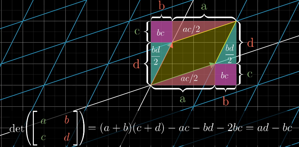
二阶行列式
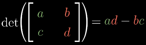
$\begin{vmatrix} a_{11} & a_{12} \\ a_{21} & a_{22} \\ \end{vmatrix} = a_{11}a_{22} - a_{12}a_{21}$
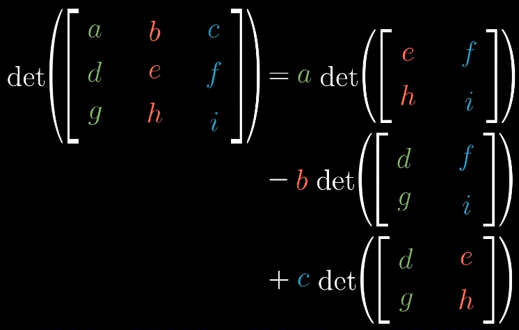
三阶行列式
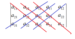
对于更高阶的行列式,一般将行列式转为三角形,这样只用计算对角线的乘积即可。
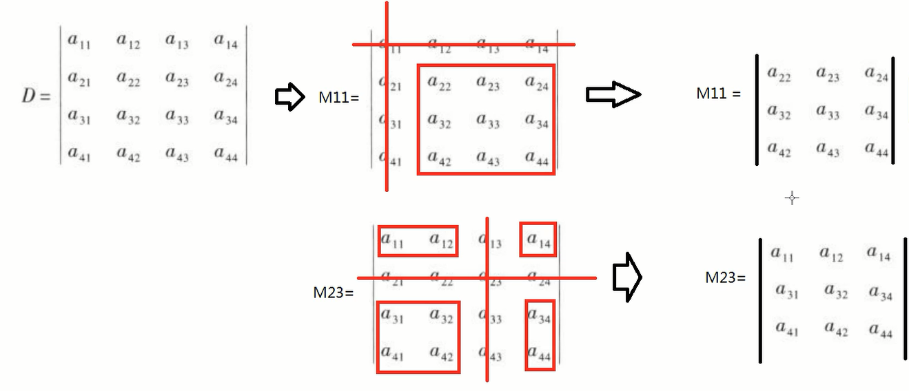
$n$阶行列式,把第$a_{ij}$所在的行列删除,留下的$n-1$阶行列式称为余子式,记为$M_{ij}$。
代数余子式的$A_{ij} = -1^{i+j}M_{ij}$。
代数余子式的转置称为伴随矩阵,只有方阵才有伴随矩阵,记为$A^*$。
伴随矩阵的性质:
$AA^* = A^*A = |A|E$
$A^{-1} = \frac{1}{|A|}A^*(存在A^{-1})$
$(A^*)^{-1}=(A^{-1})^*=\frac{1}{|A|}A$
$|A^*|=|A|^{n-1}$
$(kA)^*=k^{n-1}A^*$
$A^{-1} = \frac{1}{|A|}A^*(存在A^{-1})$
$A^{-1} = \frac{1}{|A|}A^{*}=\frac{1}{ad-bc}\begin{bmatrix}d &-b\ -c & a\end{bmatrix}$
例:
向量对于不同的学科有不一样的定义。
物理中的向量有长度和方向决定,长度和方向不变可以随意移动,它们表示的是同一个向量。
计算机中的向量更多的是对数据的抽象,可以根据面积和价格定义一个房子$\begin{bmatrix}100m^2\\700000¥\end{bmatrix}$。
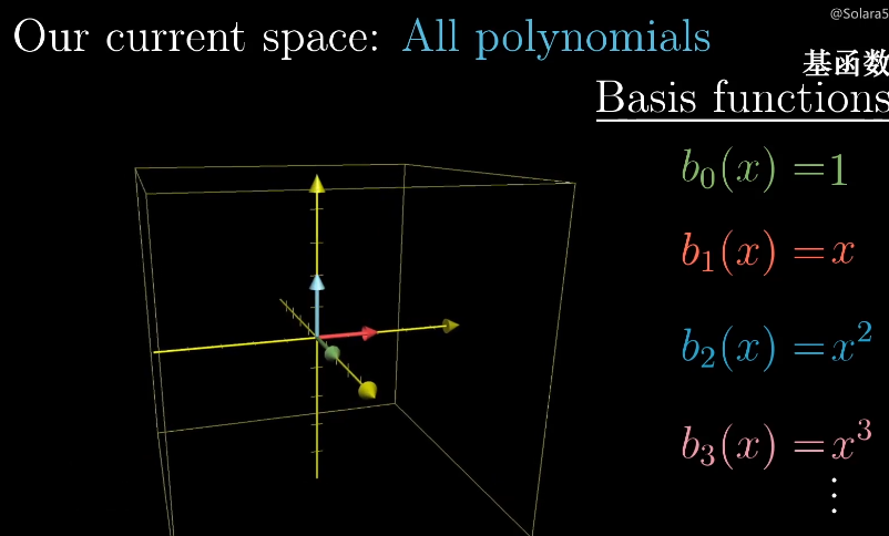
数学中的向量可以是任意东西,只要保证两个向量的相加$\vec v + \vec w$以及数字和向量相乘$2\vec v$是有意义的即可。
线性代数中的向量可以理解为一个空间中的箭头,这个箭头起点落在原点。如果空间中有许多的向量,可以点表示一个向量,即向量头的坐标。
向量的基本运算
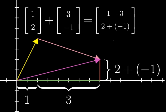
向量的加法:可以理解为在坐标中两个向量的移动。
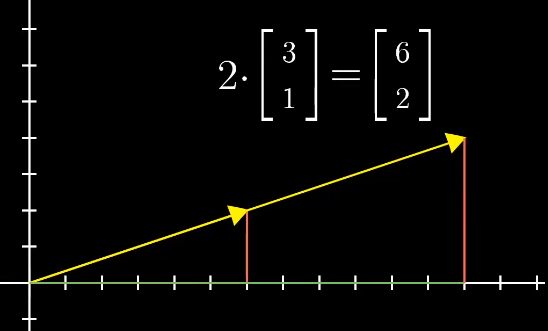
数字和向量相乘:可以理解为向量的缩放。
线性组合
两个数乘向量称为两个向量的线性组合$a\vec v+ b\vec w$。
两个不共线的向量通过不同的线性组合可以得到二维平面中的所有向量。
两个共线的向量通过线程组合只能得到一个直线的所有向量。
如果两个向量都是零向量那么它只能在原点。
张成空间
所有可以表示给定向量线性组合的向量的集合称为给定向量的张成空间(span)。
一般来说两个向量张成空间可以是直线、平面。
三个向量张成空间可以是平面、空间。
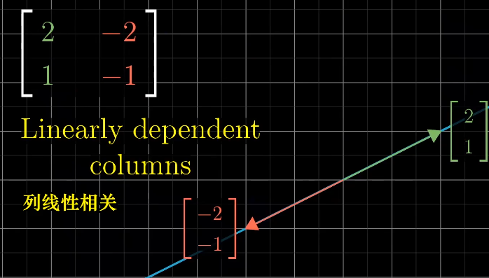
如果多个向量,并且可以移除其中一个而不减小张成空间,那么它们是线性相关的,也可以说一个向量可以表示为其他向量的线性组合$\vec u = a \vec v + b\vec w$。
如果所有的向量都给张成的空间增加了新的维度,它们就成为线性无关的$\vec u \neq a \vec v + b\vec w$。
基
向量空间的一组及是张成该空间的一个线性无关向量集。
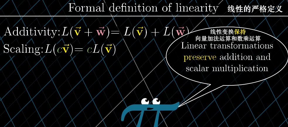
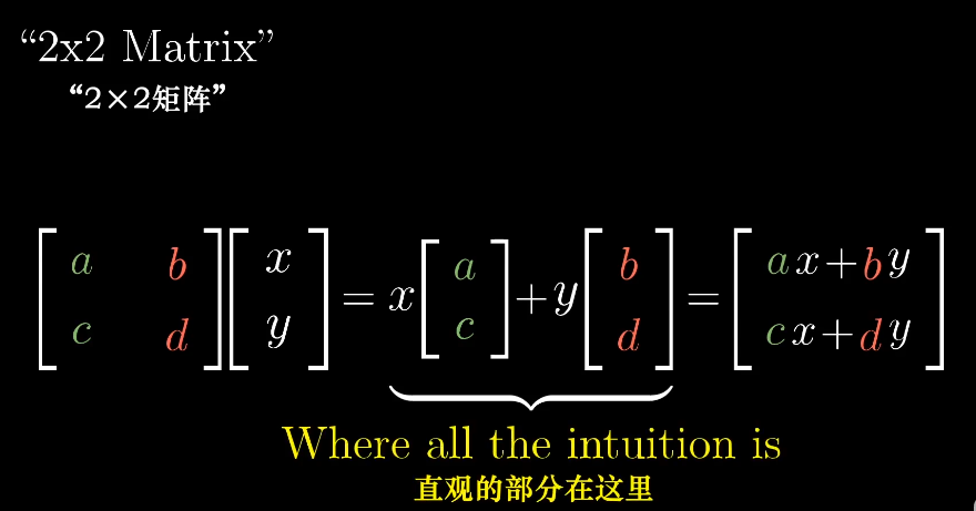
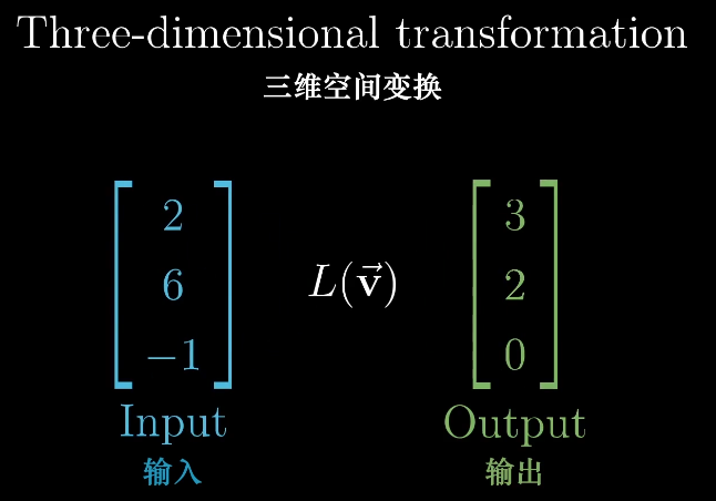
严格意义上来说,线性变换是将向量作为输入和输出的一类函数。
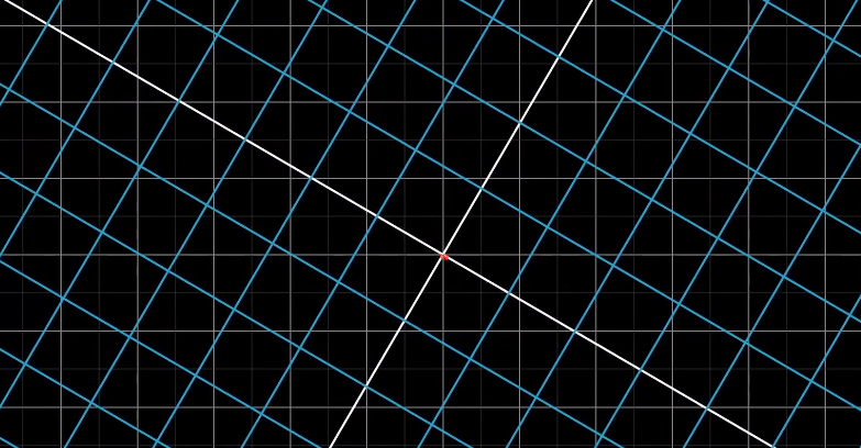
变化可以多种多样,线性变化将变化限制在一个特殊类型的变换上,可以简单的理解为网格线保持平行且等距分布。
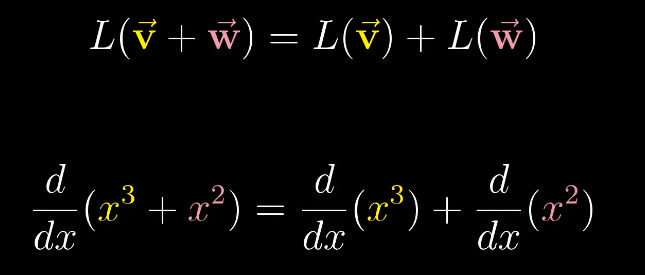
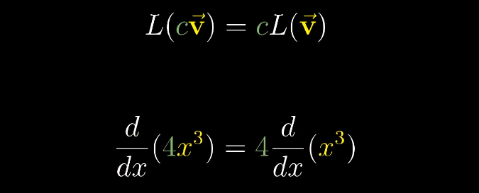
线性变化满足一下两个性质:
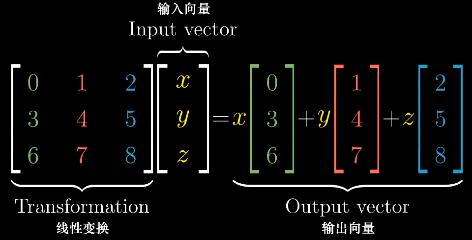
可以使用基向量来描述线性变化:
通过记录两个基向量$\hat{i}$,$\hat{j}$的变换,就可以得到其他变化后的向量。
已知向量$\vec v = \begin{bmatrix}-1\\2\end{bmatrix}$
变换之前的$\hat i$和$\hat j$:
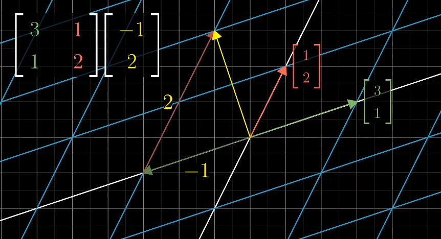
如果变化后的$\hat{i}$和$\hat{j}$是线性相关的,变化后向量的张量就是一维空间:
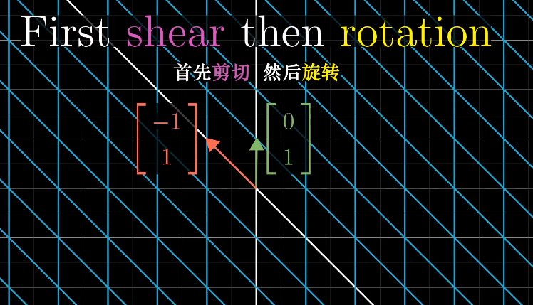
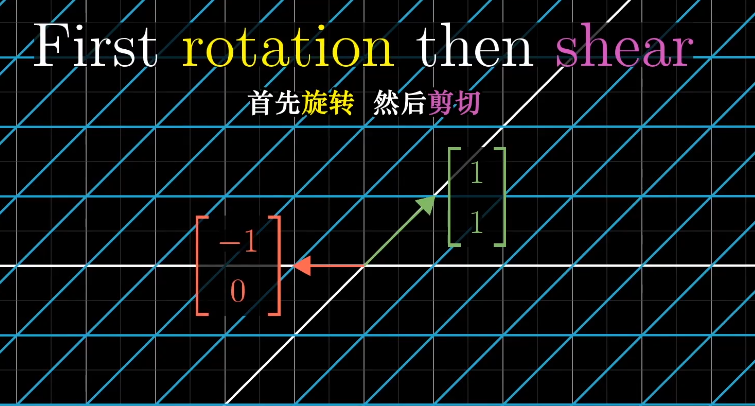
线性变化的复合
如何描述先旋转再剪切的操作呢?
一个通俗的方法是首先左乘旋转矩阵然后左乘剪切矩阵。
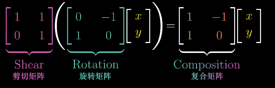
两个矩阵的乘积需要从右向左读,类似函数的复合。

这样两个矩阵的乘积就对应了一个复合的线性变换,最终得到对应变换后的$\hat{i}$和$\hat{j}$。
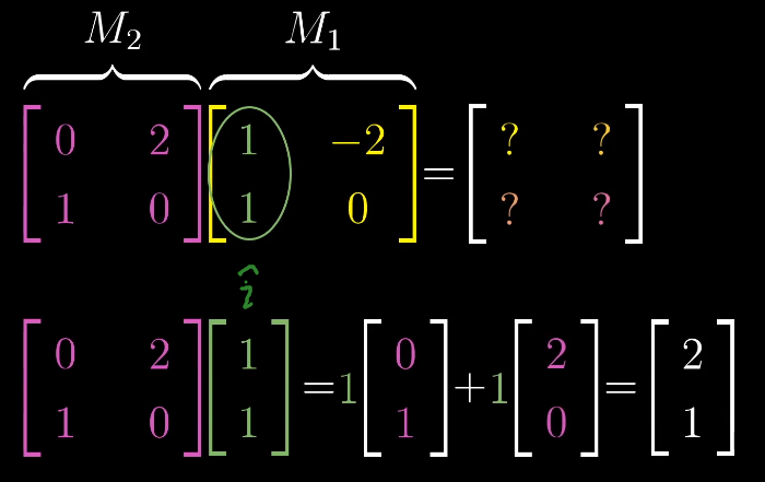
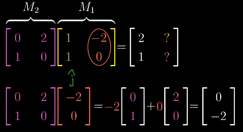
这一过程具有普适性:
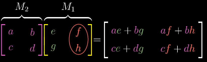
矩阵乘法的顺序
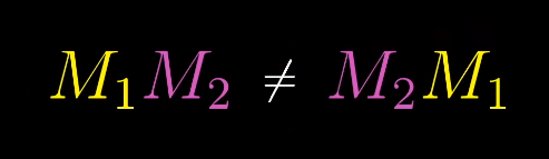
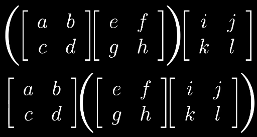
如何证明矩阵乘法的结合性?
$(AB)C = A(BC)$
根据线性变化我们可以得出,矩阵的乘法都是以CBA的顺序变换得到,所以他们本质上相同,通过变化的形式解释比代数计算更加容易理解。
三维的空间变化和二维的类似。
同样跟踪基向量的变换,能很好的解释变换后的向量,同样两个矩阵相乘也是。
行列式的本质
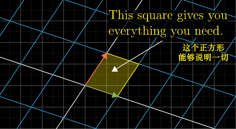
行列式的本质是计算线性变化对空间的缩放比例,具体一点就是,测量一个给定区域面积增大或减小的比例。
单位面积的变换代表任意区域的面积变换比例。
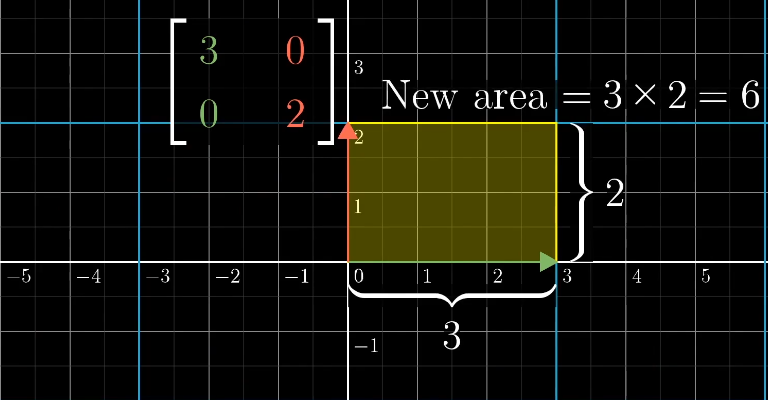
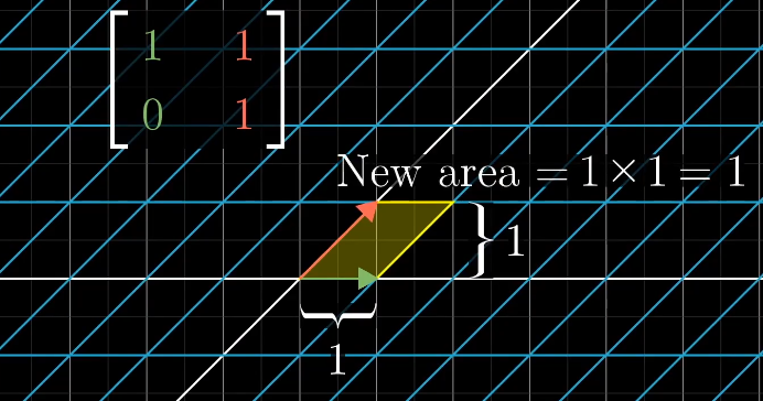
行列式的值表示缩放比例。
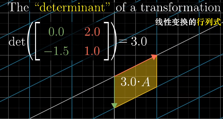
行列式为什么有负值呢?
三维空间的行列式类似,它的单位是一个单位1的立方体。
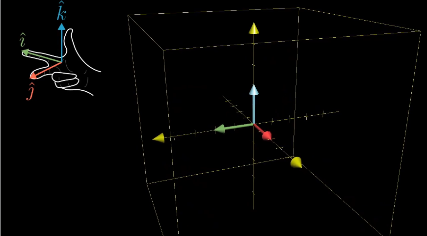
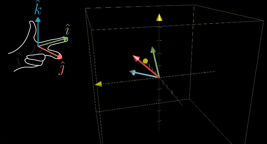
三位空间的线性变换,可以使用右手定则判断三维空间的定向。如果变换前后都可以通过右手定则得到,那么他的行列式就是正值,否则为负值。
行列式的计算
二阶行列式
三阶行列式
二阶行列式中a、d,表示横向和纵向的拉伸,b、c表示对角线的拉伸和压缩的情况。
线性方程组
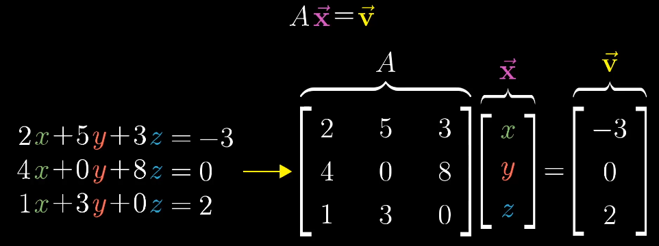
从几何的角度来思考,矩阵A表示一个线性变换,我们需要找到一个$\vec x$使得它在变换后和$\vec v$重合。
逆矩阵
矩阵的逆运算,记为$\vec A = \begin{bmatrix}3&1 \\0&2\end{bmatrix}^{-1}$,对于线程方程$A \vec x = \vec v $来说,找到$A^{-1}$就得到解$\vec x = A^{-1} \vec v$。
线性方程组的解
对于方程组$A\vec x = \vec v$,线性变换A存在两种情况:
$det(A) \neq0$:这时空间的维数并没有改变,有且只有一个向量经过线性变换后和$\vec v$重合。
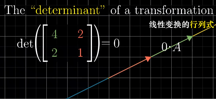
$det(A) =0$:空间被压缩到更低的维度,这时不存在逆变换,因为不能将一个直线解压缩为一个平面,这样就会映射多个向量。但是即使不存在逆变换,解可能仍然存在,因为目标$\vec v$刚好落在压缩后的空间上。
秩
秩代表变换后空间的维度。
如果线性变化后将空间压缩成一条直线,那么称这个变化的秩为1;
如果线性变化后向量落在二维平面,那么称这个变化的秩为2。
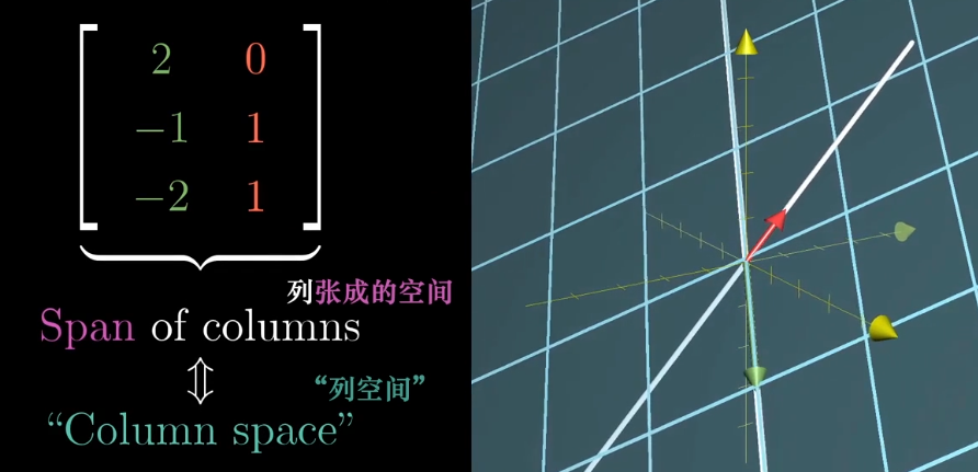
列空间
所有可能的输出向量$A\vec v$构成的集合,称为列空间,即所有列向量张成的空间。
零空间(Null space)
所有的线性变化中,零向量一定包含在列空间中,因为线性变换原点保持不动。对于非满秩的情况来说,会有一系列的向量在变换后仍为零向量。
二维空间压缩为一条直线,一条线上的向量都会落到原点。
三维空间压缩为二维平面,一条线上的向量都会落到原点。
三维空间压缩为一条直线,整个平面上的向量都会落到原点。
当$A\vec x = \vec v$中的$\vec v$是一个零向量,即$A\vec x = \begin{bmatrix}0 \\0\end{bmatrix}$时,零空间就是它所有可能的解。
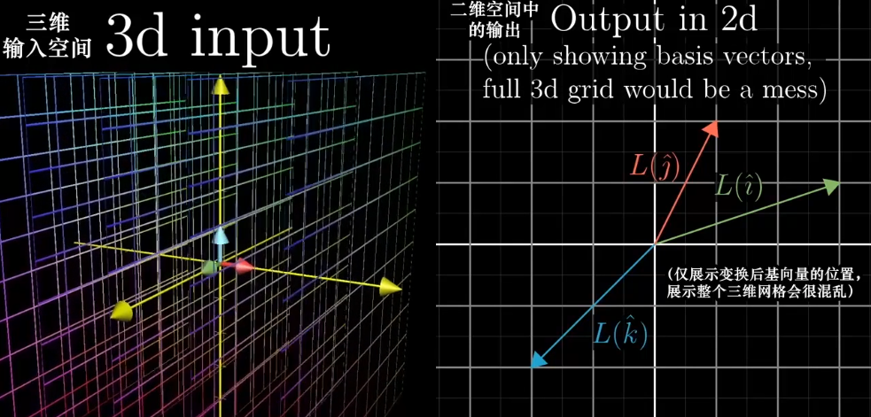
不同维度的变换也是存在的。
一个$3\times2$的矩阵:$\begin{bmatrix}2&0\-1&1\-2&1 \end{bmatrix}$它的集合意义是将一个二维空间映射到三维空间上,矩阵有两列表明输入空间有两个基向量,有三行表示每个向量在变换后用三个独立的坐标描述。
一个$2\times 3$的矩阵:$\begin{bmatrix}3&1&4\1&5&9 \end{bmatrix}$则表示将一个三维空间映射到二维空间上。
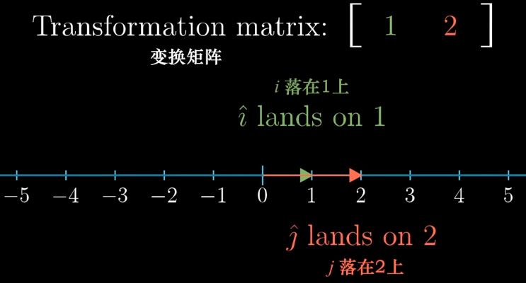
一个$1\times 2$的矩阵:$\begin{bmatrix}1&2 \end{bmatrix}$表示一个二维空间映射到一维空间。
点积
对于两个维度相同的向量,他们的点积计算为:$\begin{bmatrix}1\\2\end{bmatrix}\cdot\begin{bmatrix} 3\\4\end{bmatrix}=1\cdot3+2\cdot4=11$。
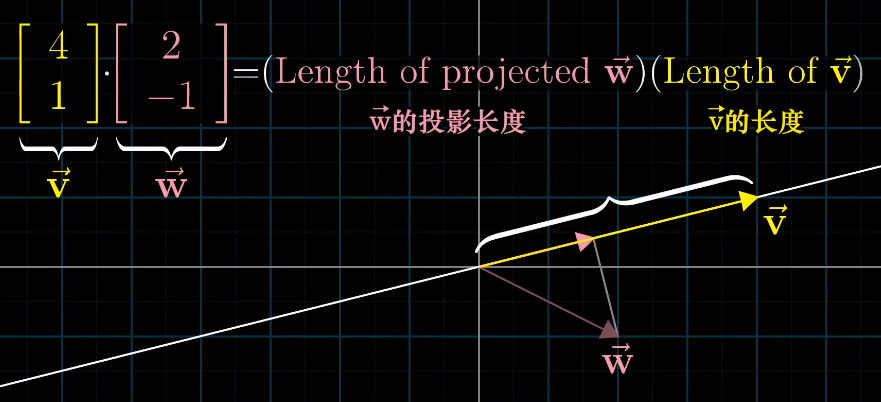
点积的几何解释是将一个向量向一个向量投影,然后两个长度相乘,如果为负数则表示反向。
为什么点积和坐标相乘联系起来了?这和对偶性有关。
对偶性
对偶性的思想是:每当看到一个多维空间到数轴上的线性变换时,他都与空间中的唯一一个向量对应,也就是说使用线性变换和与这个向量点乘等价。这个向量也叫做线性变换的对偶向量。
当二维空间向一维空间映射时,如果在二维空间中等距分布的点在变换后还是等距分布的,那么这种变换就是线性的。
假设有一个线性变换A$\begin{bmatrix}1&-2\end{bmatrix}$和一个向量$\vec v=\begin{bmatrix}4\\3\end{bmatrix}$。
变换后的位置为$\begin{bmatrix}1&-2\end{bmatrix}\begin{bmatrix}4\\3\end{bmatrix}=4\cdot1+3\cdot-2=-2$,这个变换是一个二维空间向一维空间的变化,所以变换后的结果为一个坐标值。
我们可以看到线性变换的计算过程和向量的点积相同$\begin{bmatrix}1\\-2\end{bmatrix}\cdot\begin{bmatrix}4\\3\end{bmatrix}=4\cdot1+3\cdot-2=-2$,所以向量和一个线性变化有着微妙的联系。
假设有一个倾斜的数轴,上面有一个单位向量$\vec v$,对于任意一个向量它在数轴上的投影都是一个数字,这表示了一个二维向量到一位空间的一种线性变换,那么如何得到这个线性变化呢?
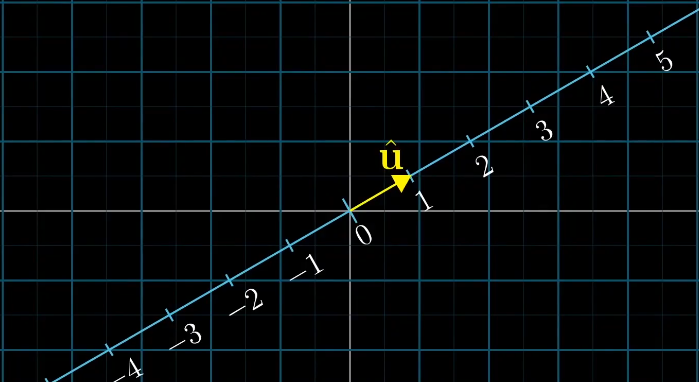
由之前的内容来说,我们可以观察基向量$\vec i$和$\vec j$的变化,从而得到对应的线性变化。
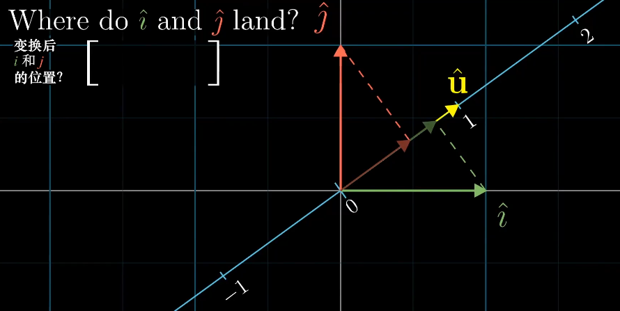
因为$\vec i$、$\vec j$、$\vec u$都是单位向量,根据对称性可以得到$\vec i$和$\vec j$在$\vec u$上的投影长度刚好是$\vec u$的坐标。
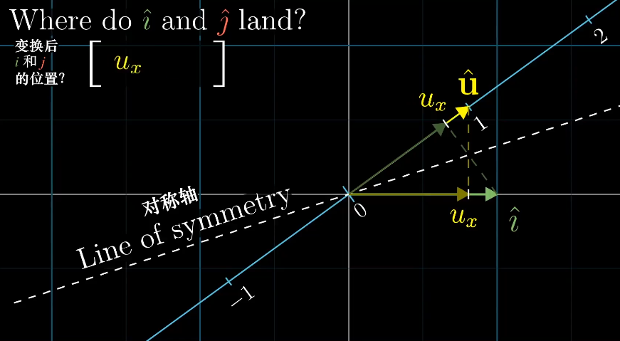
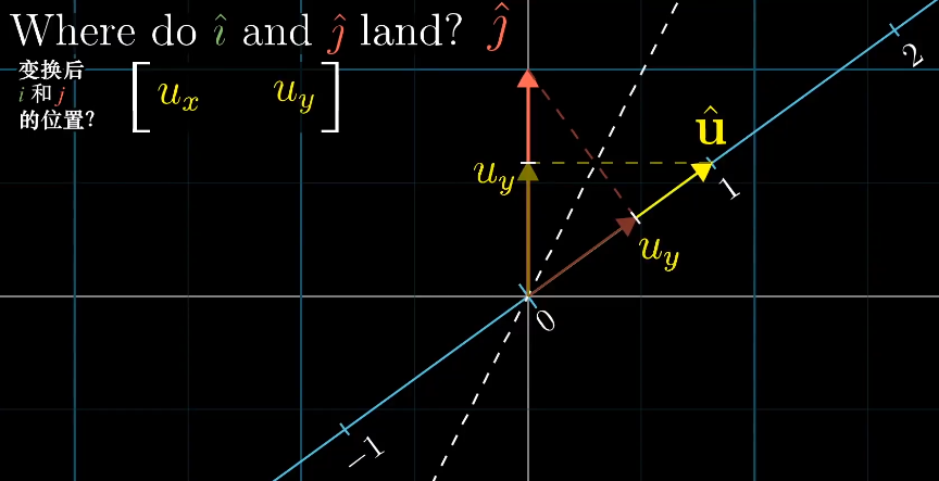
这样空间中的所有向量都可以通过线性变化$\begin{bmatrix}u_x&u_y \end{bmatrix}$得到,而这个计算过程刚好和单位向量的点积相同。
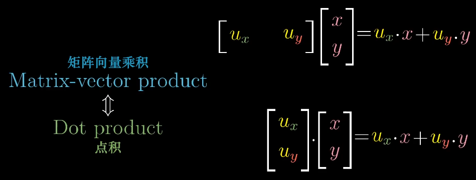
也就是为什么向量投影到直线的长度,刚好等于它与直线上单位向量的点积,对于非单位向量也是类似,只是将其扩大到对应倍数。
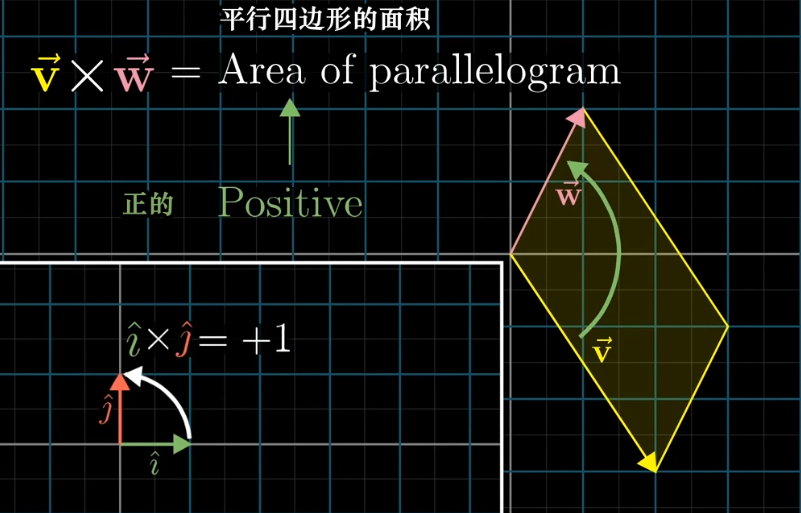
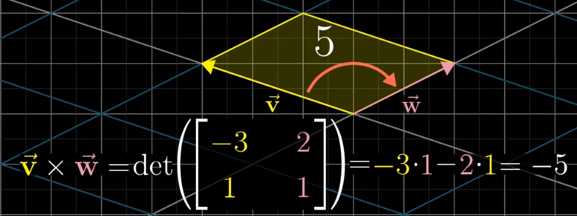
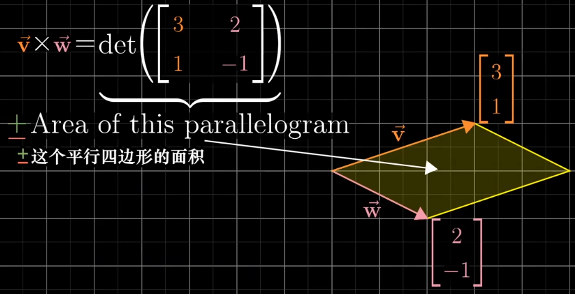
对于两个向量所围成的面积来说,可以使用行列式计算,将两个向量看作是变换后的基向量,这样通过行列式就可以得到变换后面积缩放的比例,因为基向量的单位为1,所以就得到了对应的面积。
考虑到正向,这个面积的值存在负值,这是参照基向量$\vec i$和$\vec j$的相对位置来说的。
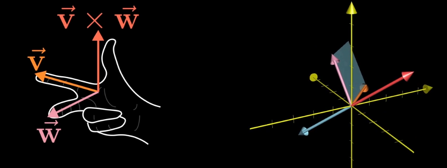
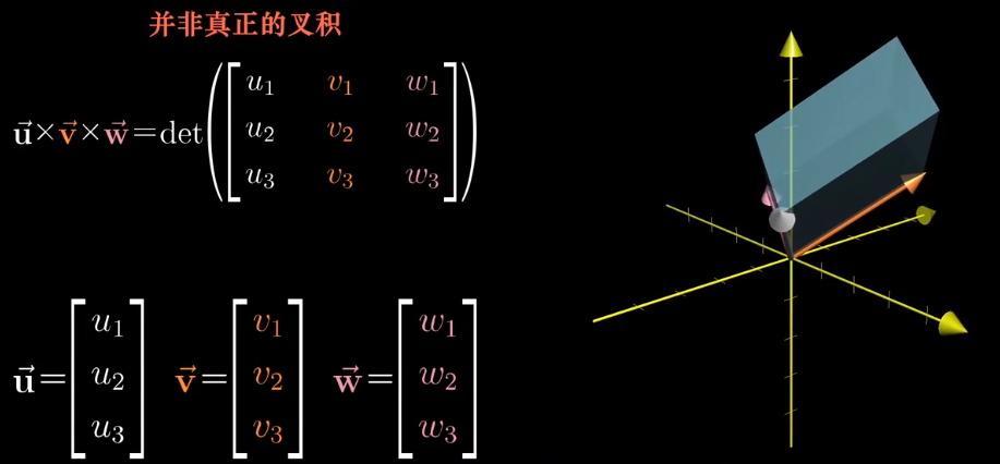
真正的叉积是通过两个三维向量$\vec v$和$\vec w$,生成一个新的三维向量$\vec u$,这个向量垂直于向量$\vec v$和$\vec w$所在的平面,长度等于它们围成的面积。
叉积的反向可以通过右手定则判断:
叉积的计算方法:
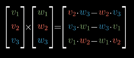
参考二维向量的叉积计算:
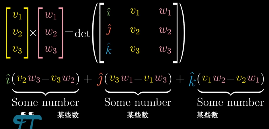
三维的可以写成类似的形式,但是他并是真正的叉积,不过和真正的叉积已经很接近了。
我可以构造一个函数,它可以把一个三维空间映射到一维空间上。
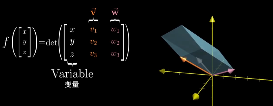
右侧行列式是线性的,所以我们可以找到一个线性变换代替这个函数。
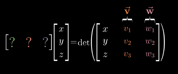
根据对偶性的思想,从多维空间到一维空间的线性变换,等于与对应向量的点积,这个特殊的向量$\vec p$就是我们要找的向量。
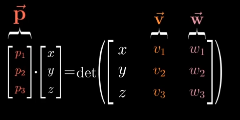
从数值计算上:
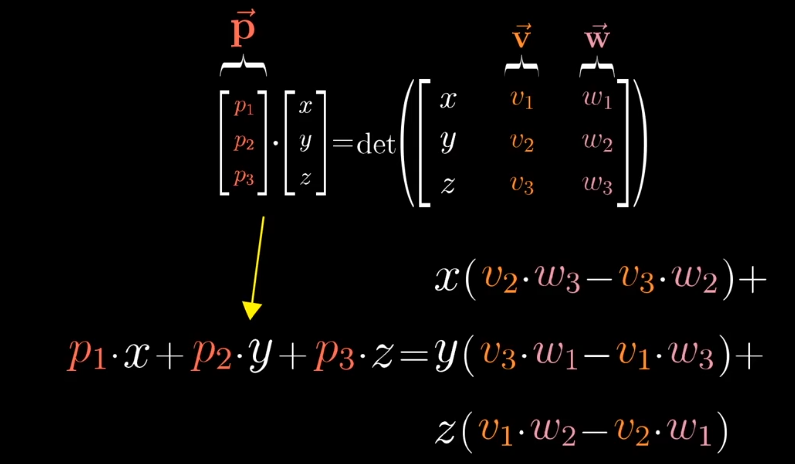
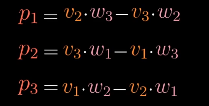
向量$\vec p$的计算结果刚好和叉积计算的结果相同。
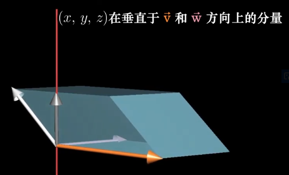
从几何意义:
当向量$\vec p$和向量$\begin{bmatrix}x\y\z \end{bmatrix}$点乘时,得到一个$\begin{bmatrix}x\y\z \end{bmatrix}$与$\vec v$与$\vec w$确定的平行六面体的有向体积,什么样的向量满足这个性质呢?
点积的几何解释是,其他向量在$\vec p$上的投影的长度乘以$\vec p$的长度。
对于平行六面体的体积来说,它等于$\vec v$和$\vec w$所确定的面积乘以$\begin{bmatrix}x\y\z \end{bmatrix}$在垂线上的投影。
那么$\vec p$要想满足这一要求,那么它就刚好符合,长度等于$\vec v,\vec w$所围成的面积,且刚好垂直这个平面。
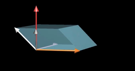
标准坐标系的基向量为$\vec {i}: \begin{bmatrix}1\\0 \end{bmatrix}$和$\vec {j}: \begin{bmatrix}0\\1 \end{bmatrix}$,假如詹妮弗有另一个坐标系:她的基向量为$\vec i \begin{bmatrix}2\\1 \end{bmatrix}$和$\vec j \begin{bmatrix}-1\\1 \end{bmatrix}$。
对于同一个点$\begin{bmatrix}3\\2 \end{bmatrix}$来说他们所表示的形式不同,在詹妮弗的坐标系中表示为$\begin{bmatrix}\frac{5}{3}\\\frac{1}{3} \end{bmatrix}$。
从标准坐标到詹尼佛的坐标系,我能可以得到一个线性变换$A:\begin{bmatrix}2&-1\\1&1 \end{bmatrix}$。
如果想知道詹妮弗的坐标系中点$\begin{bmatrix}3\\2 \end{bmatrix}$在标准坐标系的位置,可以通过$\begin{bmatrix}2&-1\\1&1 \end{bmatrix}\begin{bmatrix}3\\2 \end{bmatrix}$得到。
如果想知道标准坐标系中点$\begin{bmatrix}3\\2 \end{bmatrix}$在詹妮弗坐标系的位置,可以通过$\begin{bmatrix}2&-1\\1&1 \end{bmatrix}^{-1}\begin{bmatrix}3\\2 \end{bmatrix}$得到。
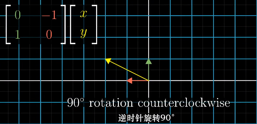
具体的例子,90°旋转。
在标准坐标系可以跟踪基向量的变化来体现:
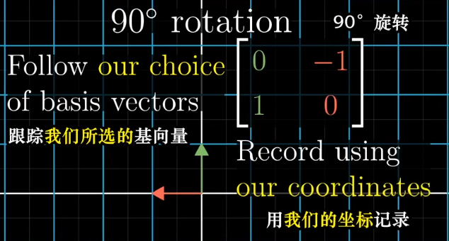
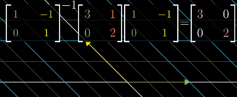
在詹妮弗的坐标系中如何表示旋转呢?首先将向量转换为标准坐标系的表示,然后左旋,最后再转换为詹妮弗的表示。
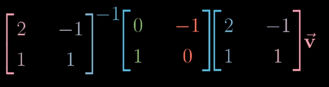
所以我们可以得到对于詹妮弗坐标系的左旋线性变化的表示:
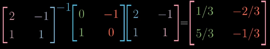
所以表达式$A^{-1}MA$表示一种数学上的转移作用,$M$表示一种线性变换,$A$和$A^{-1}$表示坐标系的转换。
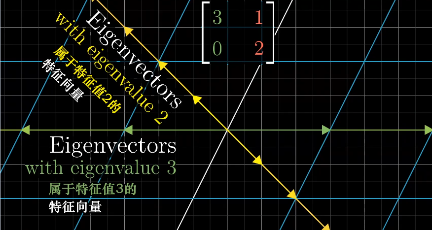
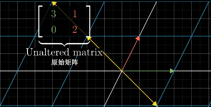
对于一些线性变化来说,存在一些向量在变换前后留在了张成的空间里,只是拉伸或收缩了一定比例,这些向量称为特征向量,拉伸收缩的比例称为特征值。
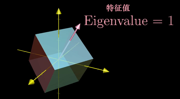
一个三维空间的旋转,如果能找到特征值为1的特征向量,那么它就是旋转轴,因为旋转并不进行缩放,且旋转轴在线性变换中保持不变。
特征向量的求解
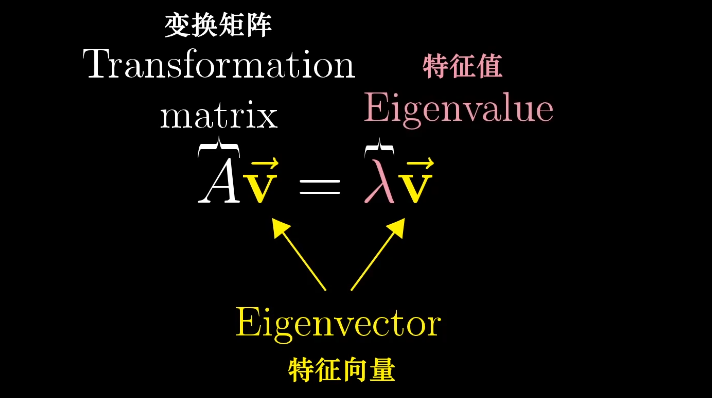
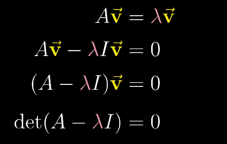
特征向量的概念,等号左侧表示矩阵向量的乘积,等号右侧表示向量数乘,可以将右侧重写为某个向量的乘积,$\vec I$为单位向量。
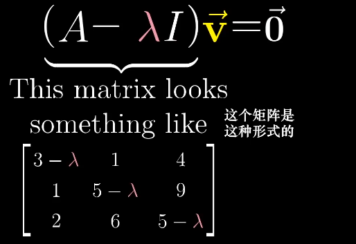
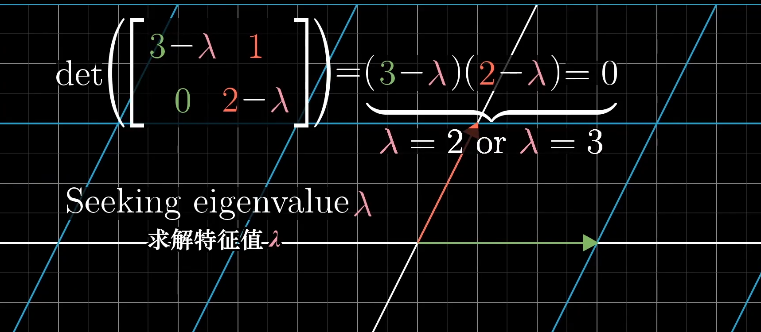
求解等式,就是使左侧的行列式det为0,$\lambda$就是特征值。
求解$\lambda$对应的特征向量时,即求解满足$(A-\lambda I)\vec{X}=0$的所有向量$\vec{X}$。
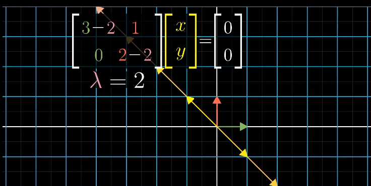
对应原始矩阵上所有落在$\begin{bmatrix} -1 \ 1 \end{bmatrix}$的向量被拉伸了2倍。
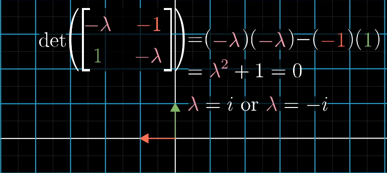
二维线性变换不一定存在特征向量,例如左旋90°,每个想都都发生了旋转,离开了张成空间。如果强行计算,会得到两个虚根:
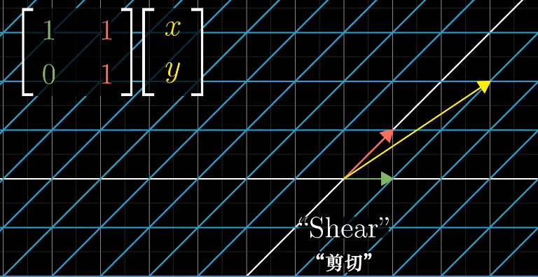
剪切变换的特征向量分布在x轴:
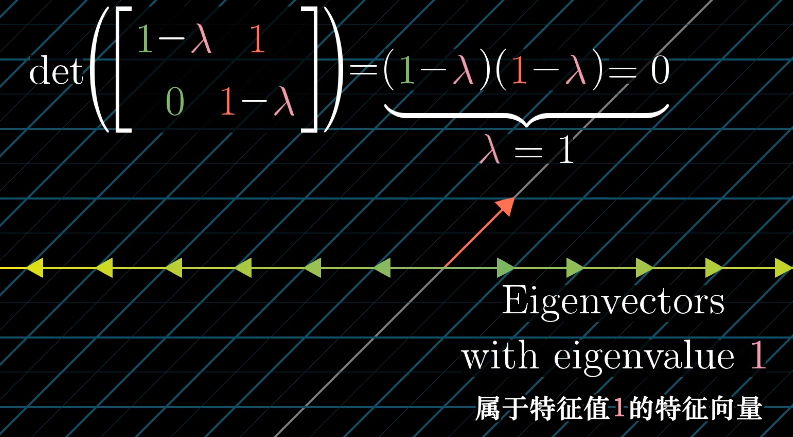
只有一个特征值,但是特征向量不一定只在一条直线上:
特征基
一组基向量构成的集合被称为一组特征基
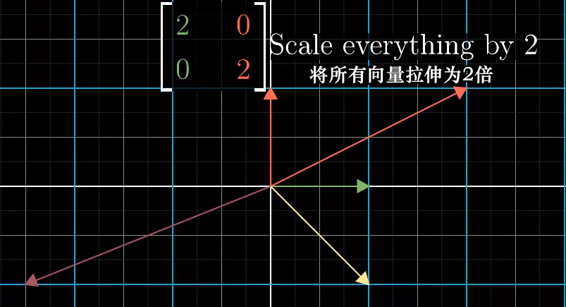
如果特征向量是基向量,它对应的矩阵是一个对角矩阵,矩阵的对角元是它们所属的特征值。
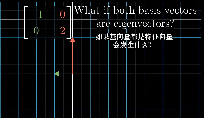
对角矩阵在求幂次时更方便求解,对应的幂次就是对角元的幂次。
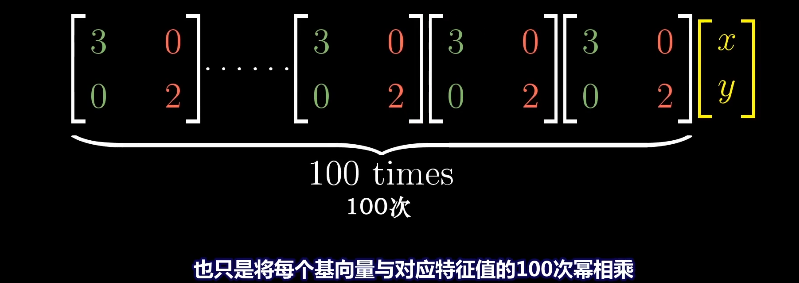
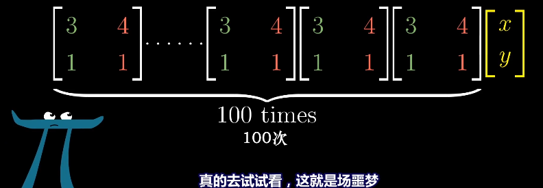
而对于非对角矩阵的幂次求解就非常麻烦。
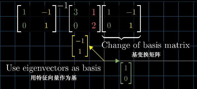
实际遇到对角矩阵的概率很低,但是我们可以通过基坐标变换来得到对角矩阵,前提有足够多的特征向量且可以张成整个空间,例如剪切变化就不行,应为它只有一个特征向量,无法进行坐标变换。
求解特征值:
$\begin{bmatrix}-\lambda&1\1&1-\lambda \end{bmatrix}\vec{X}=0$
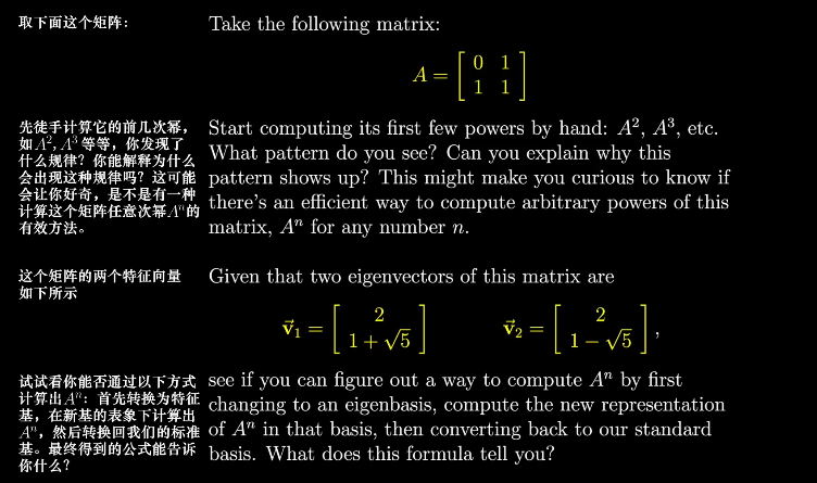
Polynomial is of great interest in various fields, such as analysis, geometry and algebra. Given a polynomial, we try to extract as many information as possible. For example, given a polynomial, we certainly want to find its roots. However this is not very realistic. Abel-Ruffini theorem states that it is impossible to solve polynomials of degree $\ge 5$ in general. For example, one can always solve the polynomial $x^n-1=0$ for arbitrary $n$, but trying to solve $x^5-x-1=0$ over $\mathbb{Q}$ is not possible. Galois showed that the flux of solvability lies in the structure of the Galois group, depending on whether it is solvable group-theoretically.
In this post, we will explore the theory of solvability in the modern sense, considering extensions of arbitrary characteristic rather than solely number fields over $\mathbb{Q}$.
Definition 1. Let $E/k$ be a separable and finite field extension, and $K$ the smallest Galois extension of $k$ containing $E$. We say $E/k$ is solvable if $G(K/k)$ (the Galois group of $K$ over $k$) is solvable.
Throughout we will deal with separable extensions because without this assumption one will be dealing with normal extensions instead of Galois extensions. Although we will arrive at a similar result.
Proposition 1. Let $E/k$ be a separable extension. Then $E/k$ is solvable if and only if there exists a solvable Galois extension $L/k$ such that $k \subset E \subset L$.
Proof. If $E/k$ is solvable, it suffices to take $L$ to be the smallest Galois extension of $k$ containing $E$. Conversely, Suppose $L/k$ is a solvable and Galois such that $k \subset E \subset L$. Let $K$ be the smallest Galois extension of $k$ containing $E$, i.e. we have $k \subset E \subset K \subset L$. We see $G(K/k) \cong G(L/k)/G(L/K)$ is a homomorphism image of $G(L/k)$ and it has to be solvable. $\square$
Next we introduce an important concept concerning field extensions.
Definition 2. Let $\mathcal{C}$ be a certain class of extension fields $F \subset E$. We say that $\mathcal{C}$ is distinguished if it satisfies the following conditions:
- Let $k \subset F \subset E$ be a tower of fields. The extension $k \subset E$ is in $\mathcal{C}$ if and only if $k \subset F$ is in $\mathcal{C}$ and $F \subset E$ is in $\mathcal{C}$.
- If $k \subset E$ is in $\mathcal{C}$ and if $F$ is any given extension of $k$, and $E,F$ are both contained in some field, then $F \subset EF$ is in $\mathcal{C}$ too. Here $EF$ is the compositum of $E$ and $F$, i.e. the smallest field that contains both $E$ and $F$.
- If $k \subset F$ and $k \subset E$ are in $\mathcal{C}$ and $F,E$ are subfields of a common field, then $k \subset FE$ is in $\mathcal{C}$.
When dealing with several extensions at the same time, it can be a great idea to consider the class of extensions they are in. For example, Galois extension is not distinguished because normal extension does not satisfy 1. That’s why we need to have the fundamental theorem of Galois theory, a.k.a. Galois correspondence, because not all intermediate subfields are Galois. Separable extension is distinguished however. We introduce this concept because:
Proposition 2. Solvable extensions form a distinguished class of extensions. (N.B. these extensions are finite and separable by default.)
Proof. We verify all three conditions mentioned in definition 2. To make our proof easier however, we first verify 2.
Step 1. Let $E/k$ be solvable. Let $F$ be a field containing $k$ and assume $E, F$ are subfields of some algebraically closed field. We need to show that $EF/F$ is solvable. By proposition 1, there is a Galois solvable extension $K/k$ such that $K \supset E \supset k$. Then $KF$ is Galois over $F$ and $G(KF/F)$ is a subgroup of $G(K/k)$. Therefore $KF/F$ is a Galois solvable extension and we have $KF \supset EF \supset F$, which implies that $EF/F$ is solvable.
Step 2. Consider a tower of extensions $E \supset F \supset k$. Assume now $E/k$ is solvable. Then there exists a Galois solvable extension $K$ containing $E$, which implies that $F/k$ is solvable because $K \supset F$. We see $E/F$ is also solvable because $EF=E$ and we are back to step 1.
Conversely, assume that $E/F$ is solvable and $F/k$ is solvable. We will find a solvable extension $M/k$ containing $E$. Let $K/k$ be a Galois solvable extension such that $K \supset F$, then $EK/K$ is solvable by step 1. Let $L$ be a Galois solvable extension of $K$ containing $EK$. If $\sigma$ is any embedding of $L$ over $k$ in a given algebraic closure, then $\sigma K = K$ and hence $\sigma L$ is a solvable extension of $K$. [This sentence deserves some explanation. Notice that $L/k$ is not necessarily Galois, therefore $\sigma$ is not necessarily an automorphism of $L$ and $\sigma L \ne L$ in general . However, since $K/k$ is Galois, the restriction of $\sigma$ on $K$ is an automorphism so therefore $\sigma K = K$. The extension $\sigma L / \sigma K$ is solvable because $\sigma L$ is isomorphic to $L$ and $\sigma K = K$.]
We let $M$ be the compositum of all extensions $\sigma L$ for all embeddings $\sigma$ of $L$ over $k$. Then $M/k$ is Galois and so is $M/K$ [note: this is the property of normal extension; besides, $M/k$ is finite]. We have $G(M/K) \subset \prod_{\sigma}G(\sigma L/K)$ which is a product of solvable groups. Therefore $G(M/K)$ is solvable, meaning $M/K$ is a solvable extension. We have a surjective homomorphism $G(M/k) \to G(K/k)$ (given by $\sigma \mapsto \sigma|_K$) and therefore $G(M/k)$ has a normal subgroup whose factor group is solvable, meaning $G(M/k)$ is solvable. Since $E \subset M$, we are done.
Step 3. If $F/k$ and $E/k$ are solvable and $E,F$ are subfields of a common field, we need to show that $EF$ is solvable over $k$. By step 1, $EF/F$ is solvable. By step 2, $EF/k$ is solvable. $\square$
Definition 2. Let $F/k$ be a finite and separable extension. We say $F/k$ is solvable by radicals if there exists a finite extension $E$ of $k$ containing $F$, and admitting a tower decomposition
such that each step $E_{i+1}/E_i$ is one of the following types:
- It is obtained by adjoining a root of unity.
- It is obtained by adjoining a root of a polynomial $X^n-a$ with $a_i \in E_i$ and $n$ prime to the characteristic.
- It is obtained by adjoining a root of an equation $X^p-X-a$ with $a \in E_i$ if $p$ is the characteristic $>0$.
For example, $\mathbb{Q}(\sqrt{-2})/\mathbb{Q}$ is solvable by radicals. We consider the polynomial $f(x)=x^2-2x+3$. We know its roots are $x_1=-1-\sqrt{-2}$ and $x_2=-1+\sqrt{-2}$. However let’s see the question in the sense of field theory. Notice that
Therefore $f(x)=0$ is equivalent to $(x-1)^2=-2$. Then $x-1=\sqrt{-2}$ and $x-1=-\sqrt{-2}$ in $\mathbb{Q}(\sqrt{-2})$ are two equations that make perfect sense. Thus we obtain our desired roots. The field gives us the liberty of basic arithmetic, and the radical extension gives us the method to look for a radical root.
It is immediate that the class of extensions solvable by radicals is a distinguished class.
In general, we are adding “$n$-th root of something”. However, when the characteristic of the field is not zero, there are some complications. For example, talking about the $p$-th root of an element in a field of characteristic $p>0$ will not work. Therefore we need to take good care of that. The second and third types are nods to Kummer theory and Artin-Schreier theory respectively, which are deduced from Hilbert’s theorem 90’s additive and multiplicative form. We interrupt the post by introducing the respective theorems.
Let $K/k$ be a cyclic extension of degree $n$, that is, $K/k$ is Galois and $G(K/k)$ is cyclic. Suppose $G(K/k)$ is generated by $\sigma$. Then we have the celebrated “Theorem 90”:
Theorem 1 (Hilbert’s theorem 90, multiplicative form). Notation being above, let $\beta \in K$. The norm $N_{k}^{K}(\beta)=1$ if and only if there exists an element $\alpha \ne 0$ in $K$ such that $\beta = \alpha/\sigma\alpha$.
To prove this, we need Artin’s theorem of independent characters. With this, we see the second type of extension in definition 2 is cyclic.
Theorem 2. Let $k$ be a field, $n$ an integer $>0$ prime to the characteristic of $k$, and assume that there is a primitive $n$-th root of unity in $k$.
- Let $K$ be a cyclic extension of degree $n$. Then there exists $\alpha \in K$ such that $K = k(\alpha)$ and $\alpha$ satisfies an equation $X^n-a=0$ for some $a \in k$.
- Conversely, let $a \in k$. Let $\alpha$ be a root of $X^n-a$. Then $k(\alpha)$ is cyclic over $k$ of degree $d|n$, and $\alpha^d$ is an element of $k$.
All in all, theorem 2 states that a $n$-th root of $a$ yields a cyclic extension. However we don’t drop the assumption that $n$ is prime to the characteristic of $k$. When this is not the case, we will use Artin-Schreier theorem.
Theorem 3 (Hilbert’s theorem 90, additive form). Let $K/k$ be a cyclic extension of degree $n$. Let $\sigma$ be the generator of $G(K/k)$. Let $\beta \in K$. The trace $\mathrm{Tr}_k^K(\beta)=0$ if and only if there exists an element $\alpha \in K$ such that $\beta = \alpha-\sigma\alpha$.
This theorem requires another application of the independence of characters.
Theorem 4 (Artin-Schreier). Let $k$ be a field of characteristic $p$.
- Let $K$ be a cyclic extension of $k$ of degree $p$. Then there exists $\alpha \in K$ such that $K=k(\alpha)$ and $\alpha$ satisfies an equation $X^p-X-a=0$ with some $a \in k$.
- Conversely, given $a \in k$, the polynomial $f(X)=X^p-X-a$ either has one root in $k$, in which case all its roots are in $k$, or it is irreducible. In the latter case, if $\alpha$ is a root then $k(\alpha)$ is cyclic of degree $p$ over $k$.
In other words, instead of looking at the $p$-th root of unity in a field of characteristic $p$, we look at the root of $X^p-X-a$, which still yields a cyclic extension.
Now we are ready for the core theorem of this post.
Theorem 5. Let $E$ be a finite separable extension of $k$. Then $E$ is solvable by radicals if and only if $E/k$ is solvable.
Proof. First of all we assume that $E/k$ is solvable. Then there exists a finite Galois solvable extension of $k$ containing $E$ and we call it $K$. Let $m$ be the product of all primes $l$ such that $l \ne \operatorname{char}k$ but $l|[K:k]$. Let $F=k(\zeta)$ where $\zeta$ is a primitive $m$-th root of unity. Then $F/k$ is abelian and is solvable by radical by definition.
Since solvable extensions form a distinguished class, we see $KF/F$ is solvable. There is a tower of subfields between $F$ and $KF$ such that each step is cyclic of prime order, because every solvable group admits a tower of cyclic groups, and we can use Galois correspondence. By theorem 2 and 4, we see $KF/F$ is solvable by radical because extensions of prime order have been determined by these two theorems. It follows that $E/k$ is solvable by radicals: $KF/F$ is solvable by radicals, $F/k$ is solvable by radicals $\implies$ $KF/k$ is solvable by radicals $\implies$ $E/k$ is solvable by radicals because $KF \supset E \supset k$.
The elaboration of the “if” part is as follows. In order to prove $E/k$ is solvable by radicals, we show that there is a much bigger field $KF$ containing $E$ such that $KF/k$ is solvable by radical. First of all there exists a finite Galois solvable extension $K/k$ containing $E$. Next we define a cyclotomic extension $F/k$ with the following intentions
To reach these two goals, we decide to put $F=k(\zeta)$ where $\zeta$ is a $m$-th root of unity and $m$ is the radical of $[K:k]$ divided by the characteristic of $k$ when necessary. This field $F$ certainly ensures that $F/k$ is solvable by radical. For the second goal, we need to take a look of the subfield between $F$ and $KF$. Let $k = K_0 \subset K_1 \subset \dots \subset K_n = K$ be a tower of field extensions such that every step $K_{i+1}/K_i$ is of prime degree [this is possible due to the solvability of $K/k$]. These prime numbers can only be factors of $[K:k]$ Then in the lifted field extension $F=K_0F \subset K_1F \subset \dots \subset K_nF=KF$ we do not introduce new prime numbers. Why do we consider prime factors of $[K:k]$? Let’s say $[K_{i+1}F:K_iF] = \ell$ is a prime number. If $\ell=\operatorname{char}k$ then we can use theorem 4. Otherwise we still have $\ell|[K:k]$ so we use theorem 2. However this theorem requires a primitive $\ell$-th root to be in $K_{i}F$. Our choice of $m$ and $\zeta$ guaranteed this to happen because $\ell|m$ and therefore a primitive $\ell$-th root of unity exists in $F$. We can make $m$ bigger but there is no necessity. The “only if” part does nearly the same thing, with an alternation of logic chain.
Conversely, assume that $E/k$ is solvable by radicals. For any embedding $\sigma$ of $E$ in $E^{\mathrm{a}}$ over $k$, the extension $\sigma E/k$ is also solvable by radicals. Hence the smallest Galois extension $K$ of $E$ containing $k$, which is a composite of $E$ and its conjugates is solvable by radicals. Let $m$ be the product of all primes unequal to the characteristic dividing the degree $[K:k]$ and again let $F=k(\zeta)$ where $\zeta$ is a primitive $m$-th root of unity. It will suffice to prove that $KF$ is solvable over $F$, because it follows that $KF$ is solvable by $k$ and hence $G(K/k)$ is solvable because it is a homomorphic image of $G(KF/k)$. But $KF/F$ can be decomposed into a tower of extensions such that each step is prime degree and of the type described in theorem 2 and theorem 4. The corresponding root of unity is in the field $F$. Hence $KF/F$ is solvable, proving the theorem. $\square$
There are a lot of important linear algebraic groups that are widely used in mathematics, physics and industry. Some of them have nice visualisations. For example, it is widely known that $SU(2) \cong S^3$ and $SO(3) \cong \mathbb{RP}^3$. The group $SL(2,\mathbb{R})$ is not less important than them but the visualisation concerning this group is not very easy to be found. In this post we show that
where $D$ is the open unit disk. In other words, $SL(2,\mathbb{R})$ can be considered as a donut, not the shell of it ($S^1 \times S^1$) but the “content” or “flesh” of it. More formally, the inside of a solid torus.
The related core theory can be found in Iwasawa decomposition, but to access it we need Lie group and Lie algebra theories, which involves differential geometry and certainly goes beyond the scope of this post. Interested readers can refer to Lie Groups Beyond an Introduction chapter 6 for Iwasawa decomposition theory.
Before we establish the homeomorphism
we first see what we can derive from it.
No. Since $D$ is not compact, $S^1 \times D$ cannot be compact.
Notice there is a (strong) deformation retract between $S^1 \times D$ and $S^1$. Therefore $\pi_1(SL(2,\mathbb{R})) = \pi_1(S^1)=\mathbb{Z}$.
It is connected because $S^1$ and $D$ are connected. It is not simply connected because the fundamental group is not trivial.
The dimension is $3$.
If we directly jump to the conclusion without mentioning Lie theory, one will see the decomposition comes from nowhere. Instead of defining $K$, $A$ and $N$ that will appear later and show that there is no discrepancy, we deduce the decomposition without the usage of Lie theory. Instead, we consider the action of $SL(2,\mathbb{R})$ on the upper half plane, because group action is likely to expose more information of the group.
Consider the group action of $SL(2,\mathbb{R})$ on the upper half plane
given by
Up to an explosion of calculation, one can indeed verify that this is a group action and in particular
As one may guess, it is not wise to continue without investigating the action first, or we will be lost in calculation. We first show that this action is transitive by showing that for any $z=x+yi \in \mathfrak{H}$, there is some $\sigma \in SL(2,\mathbb{R})$ such that $\sigma(z)=i$:
Let’s play around the last linear equation system:
We can put $c=0$ and $a=\frac{1}{\sqrt{y}}$ so that $b=-\frac{x}{\sqrt{y}}$ and $d=\sqrt{y}$. That is,
We have therefore proved:
The action of $SL(2,\mathbb{R})$ on $\mathfrak{H}$ is transitive.
Proof. For any $z,z’ \in \mathfrak{H}$, there exists $\sigma$ and $\sigma’$ such that $\sigma(z)=i$ and $\sigma’(z’)=i$. Then $\sigma’^{-1}(\sigma(z))=z’$, i.e. $\sigma’^{-1}\sigma$ sends $z$ to $z’$. $\square$
By working around $i$ on $\mathfrak{H}$ we can save ourselves from a lot of troubles. It is then desirable to find the stabiliser of $i$.
The stabiliser of $i \in \mathfrak{H}$ is $SO(2) \cong S^1$.
Proof. Suppose $\sigma=\begin{pmatrix} a & b \\c & d \end{pmatrix}$ stabilises $i$. Then first of all we have
Then
It follows that
Therefore $\sigma \in O(2) \cap SL(2) = SO(2)$ as expected. $\square$
With these being said, the action of $SL(2,\mathbb{R})$ on $i$ consists of $SO(2)$ that moves nothing and the rest that actually move things. In other words, $SL(2,\mathbb{R})/SO(2) \cong \mathfrak{H}$ as a $2$-manifold. In particular, the action is a isometry. We will find the effective part of the group action out. For $\sigma \in SL(2,\mathbb{R})$, we assume that $\sigma(i)=x+iy$. Then
Let $B$ be the upper triangular matrices in $SL(2,\mathbb{R})$ with positive diagonal elements. Then it is elements in $B$ that actually move things. According to this classification, we have obtained a decomposition
The matrix multiplication map $B \times SO(2) \to SL(2,\mathbb{R})$ is surjective.
Proof. Notice that every element of $B$ can be written in the form
For any $\sigma \in SL(2,\mathbb{R})$, suppose $\sigma(i)=x+iy$, then $\sigma(i)=\lambda_{x,y}(i)$, therefore $\lambda_{x,y}^{-1}\sigma(i)=i$, i.e. $\lambda_{x,y}^{-1}\sigma \in SO(2)$, i.e. $\lambda_{x,y}^{-1}\sigma$ is a stabiliser of $i$. The product $\sigma = \lambda_{x,y}(\lambda_{x,y}^{-1}\sigma)$ always lies in the image of $B \times SO(2)$. $\square$
We can decompose $B$ further:
Let $N$ be the group of upper triangular matrices in $SL(2,\mathbb{R})$ with $1$ on the diagonal line and let $A$ be the group of diagonal matrices with non-negative entries. Then $B=NA$. Let $K=SO(2) \subset SL(2,\mathbb{R})$, then we have obtained the so-called Iwasawa decomposition:
There is a diffeomorphism onto
Proof. It only remains to show injectivity. Suppose $n_1a_1k_1=n_2a_2k_2$. Applying both sides onto $i$ we obtain $n_1a_1(i)=n_2a_2(i)$. Suppose
Then we have $n_1a_1(i)=x_1+y_1i=n_2a_2(i)=x_2+y_2i$. It follows that $x_1=x_2$ and $y_1=y_2$, i.e. $n_1=n_2$ and $a_1=a_2$ and therefore $k_1=k_2$. $\square$
By investigating $N$ and $A$ further we obtain
The group $SL(2,\mathbb{R})$ is homeomorphic to $S^1 \times D$.
Proof. Notice that $N$ is homeomorphic to $\mathbb{R}$ and $A$ is homeomorphic to $\mathbb{R}_{>0}\cong \mathbb{R}$. $\square$
Notice the order of $N,A,K$ does not matter very much: $NAK,KAN,ANK,KNA$ are the same thing. This is because $AN=NA$ and for $nak \in SL(2,\mathbb{R})$, we have $(nak)^{-1}=k^{-1}a^{-1}n^{-1}$ which lies in the preimage of $K \times A \times N$ under matrix multiplication.
With the full Iwasawa decomposition in mind, we can scratch the surface of the rather complicated $SL(2,\mathbb{R})$.
The only continuous homomorphism of $SL(2,\mathbb{R})$ to $\mathbb{R}$ is trivial.
Proof. Let $f:SL(2,\mathbb{R}) \to \mathbb{R}$ be such a map. We have $f(kan)=f(k)+f(a)+f(n)$. We need to show that $f(k)=f(a)=f(n)=0$.
First of all, since $K$ is a compact subgroup of $SL(2,\mathbb{R})$, its image on $\mathbb{R}$ has to be a compact subgroup. On the other hand, $f$ on $A$ and $N$ can be constructed more explicitly. For $A$, we see $\begin{pmatrix}r & 0 \\ 0 & \frac{1}{r} \end{pmatrix} \mapsto r \mapsto \log{r}$ yields an isomorphism of $A$ and $\mathbb{R}$, in both algebraical and topological sense. For $N$ on the other hand, we immediately have an isomorphism $\begin{pmatrix}1 & x \\ 0 & 1\end{pmatrix} \mapsto x$. Therefore the image of $f$ on $A$ and $N$ can be realised as as $u\log{r}$ and $vx$ for some $u,v \in \mathbb{R}$. We use the fact that $AN=NA$ to determine $u$ and $v$. Notice that
applying $f$ on both sides, we have
For $u$, we consider the conjugate relation
Applying $f$ on both sides we obtain
This proves the triviality of $f$. $\square$
Let $f:SL(2,\mathbb{R}) \to GL(n,\mathbb{R})$ be a continuous homomorphism, then $f(SL(2,\mathbb{R})) \subset SL(n,\mathbb{R})$.
Proof. Consider the sequence of group homomorphisms
Since $SL(2,\mathbb{R})$ is connected, we see $\det\circ f(SL(2,\mathbb{R}))$ is connected, thus lying in $\mathbb{R}_{>0}$. We can then modify the sequence a little bit:
The map $\log \circ \det \circ f$ is a continuous homomorphism sending $SL(2,\mathbb{R})$ to $\mathbb{R}$, which is trivial, and therefore
This proves our assertion. $\square$
There are still a lot we can do without much Lie theory but Haar measure theory. The reader is advised to try this exercise set to see, for example, that the “volume” of $SL(2,\mathbb{R})/SL(2,\mathbb{Z})$ is $\zeta(2)$. In the references / further reading section the reader will also find a way to show that $SL(2,\mathbb{Z})\backslash SL(2,\mathbb{R})/SO(2,\mathbb{R})$ has volume $\frac{\pi}{3}$.
When studying a linear space, when some subspaces are known, we are interested in the contribution of these subspaces, by studying their sum or (inner) direct sum if possible. This philosophy can be applied to many other fields.
In the context of representation theory, say, we are given a finite group $G$, with a subgroup $H$, we want to know how a character of $H$ is related to a character of $G$, through induction if anything. Next we state the content of this post more formally.
Let $G$ be a finite group with distinct irreducible characters $\chi_1,\dots,\chi_h$. A class function $f$ on $G$ is a character if and only if it is a linear combination of the $\chi_i$’s with non-negative integer coefficients. We denote the space of characters by $R^+(G)$. However, $R^+(G)$ lacks a satisfying algebraic structure, for example, one is not even allowed to freely do subtraction. For this reason, we extend the coefficients to all of integers, by defining
An element of $R(G)$ is called a virtual character because when one coefficient of some $\chi_i$ is negative, it cannot be a character in the usual sense. Note that $R(G)$ is a finitely generated free abelian group, hence we are free to do subtraction in the normal sense.
Besides, since the product of two characters are still a character, we see $R(G)$ is a ring (not necessarily commutative). To be precise, it is a subring of the ring $F_\mathbb{C}(G)$, the ring of class functions of $G$ over $\mathbb{C}$. Furthermore, we actually have $F_\mathbb{C}(G) \cong \mathbb{C} \otimes R(G)$.
Let $H$ be a subgroup of $G$. Then the operation of restriction and induction defines homomorphisms $\mathrm{Res}:R(G) \to R(H)$ and $\mathrm{Ind}:R(H) \to R(G)$. By extending the Frobenius reciprocity linearly, still we find that $\mathrm{Res}$ and $\mathrm{Ind}$ are adjoints of each other. We also notice that the image of $\mathrm{Ind}:R(H) \to R(G)$ is a right ideal of $R(G)$. This is because, for any $\varphi \in R(H)$ and $\psi \in R(G)$, one has
But being an ideal should not be the end of our story. We want to know what happens if we consider more than one subgroups. For example, since every group is the union of all of its cyclic groups, what if we consider all cyclic subgroups of $G$? We are also interested in how all these ideals work together. This is where Artin’s theorem comes in.
Artin’s Theorem. Let $X$ be a family of subgroups of a finite group $G$. Let $\mathrm{Ind}:\oplus_{H \in X}R(H) \to R(G)$ be the homomorphism defined by the family of $\mathrm{Ind}_H^G$, $H \in X$. Then the following statements are equivalent:
(i) $G$ is the union of the conjugates of all $H \in X$. Equivalently, for any $\sigma \in G$, there is some $H \in X$ such that $H$ contains a conjugate of $\sigma$.
(ii) The cokernel of $\mathrm{Ind}:\bigoplus_{H \in X}R(H) \to R(G)$ is finite.
Example. Put $G=D_4$, the dihedral group consists of rotations ($\sigma$) and flips ($\tau$) of the square. We write
In this example we take $X=\{\langle\sigma\rangle,\langle\tau\rangle,\langle\tau\sigma\rangle\}$. First of all we put down the character table of $G$:
The character table of elements of $X$ is not difficult to carry out as they are characters of cyclic groups.
Instead of writing something like $\mathrm{Ind}_{\langle\sigma\rangle}^{D_4}\chi_1^\sigma=\chi_1+\chi_4$ manually for all characters, we put all of them in an induction-restriction table:
which yields a matrix naturally:
How to read the induction-restriction table? For example, the first column is $\langle \mathrm{Ind}_{\langle\sigma\rangle}^{D_4}\chi_1^\sigma,\chi_j\rangle$. Since $\mathrm{Ind}_{\langle\sigma\rangle}^{D_4}\chi_1^\sigma=\chi_1+\chi_4$, the column becomes $(1,0,0,1,0)$. On the other hand, the rows are indicated by the inner product with restriction. For example, since we have $\mathrm{Res}_{\langle\sigma\rangle}^{D_4}\chi_5=1$, thus $\langle\chi_4^\sigma,\mathrm{Res}_{\langle\sigma\rangle}^{D_4}\chi_5\rangle=1$ and therefore $T_{54}=1$. Induction and restriction coexist up to a transpose, which is another way to illustrate Frobenius reciprocity.
We obtain the induction map explicitly:
where the basis of $R(D_4)$ is $\chi_1,\dots,\chi_5$ and the basis of $R(\langle\sigma\rangle) \oplus R(\langle\tau\rangle) \oplus R(\langle\tau\sigma\rangle)$ is given by the second row of the induction-restriction table. By doing Gaussian elimination of rows and columns of $T$ (over $\mathbb{Z}$), i.e. changing the basis for $\mathbb{Z}^5$ and $\mathbb{Z}^8$, the matrix $T$ is reduced to the form
The image of $U$ is $\mathbb{Z} \oplus \mathbb{Z} \oplus \mathbb{Z} \oplus \mathbb{Z} \oplus 2\mathbb{Z}$, hence the cokernel of the induction map is
which is certainly finite. One can also verify that $X$ satisfies (i).
Consider the exact sequence
To show that $\mathrm{coker}(\mathrm{Ind})$ is finite (it is a finitely generated ring to begin with), it suffices to show that it suffices to see its result from tensoring with $\mathbb{Q}$, in other words, that
is a surjective map, i.e. it has trivial cokernel. This is equivalent to the surjectivity of the $\mathbb{C}$-linear map
By Frobenius reciprocity, this is on the other hand equivalent to the injectivity of
Notice that $\mathbb{C} \otimes R(G)$ is the space of class functions of $G$. For a class function $f$ of $G$, if its restriction on each $H$ is $0$, according to (i), all values of $f$ have been determined, therefore $f$ is $0$ everywhere.
Let $S$ be the union of the conjugates of the subgroups $H \in X$. Then we write elements in $\oplus_{H \in X}R(H)$ as $g=\sum_{H \in X}\mathrm{Ind}_H^G(f_H)$. It follows that $g$ always vanishes on $G \setminus S$. If (ii) holds, then
is a surjective map. Therefore class functions of $G$, i.e. elements of $\mathbb{C} \otimes R(G)$ vanish on $G \setminus S$, which forces $G \setminus S$ to be empty, i.e. $G=S$.
In another post we gave an exposition of irreducible representations of $SO(3)$, where we find ourselves studying harmonic polynomials on a sphere. In this post, we study another category of representations of $SO(3)$ that have its own significance in physics: projective representation. The result will be written as direct sums of irreducible representations of $SU(2)$ so the reader is advised to review the corresponding post. We recall that
Every irreducible unitary irreducible representation of $SU(2)$ is of the form $V_n$, where
Representation theory has a billion applications in physics. The group $SO(3)$ acts as the group of orientation-preserving orthogonal symmetries in $\mathbb{R}^3$ in an obvious way. The invariance under this action justifies the principle that physical reactions such as those between elementary particles should not depend on the observer’s vantage point.
Nevertheless, applications of representation theory in physics do not end at finite dimensional vector spaces. Put infinite dimensional vector spaces aside, we sometimes also need a class of vectors, in lieu of a single vector. For example, given a wavefunction $\psi$, we know $|\psi|^2$ has an interpretation of probability density. But then for any $\lambda \in S^1$, we see $|\lambda\psi|^2=|\psi|^2$, therefore $\lambda\psi$ and $\psi$ should be equivalent in a sense. By considering these equivalent classes, we find ourselves considering the projective space. Hence it makes sense to consider projective representations
where $G$ is compact. In this post we will assume $G=SO(3)$ and see how far we can go.
We begin with a simple group-theoretic lemma:
Lemma 1. One has
where $C_n$ is the group of $n$th roots of unity, embedded into $SL(n,\mathbb{C})$ via the map $\xi \to \xi I$.
Proof. Consider the canonical map
This map is surjective. For any $B\mathbb{C}^\ast \in GL(n,\mathbb{C})/\mathbb{C}$, we have $B\mathbb{C}^\ast=\frac{1}{|B|}B\mathbb{C}^\ast$, and $\frac{1}{|B|}B \in SL(n,\mathbb{C})$ is the preimage of $B\mathbb{C}^\ast$.
On the other hand, we see $\ker p$ consists of scalar matrices in $SL(n,\mathbb{C})$. If $\lambda I \in SL(n,\mathbb{C})$, then $|\lambda I|=\lambda^n=1$, thereby $\ker p$ can be identified as $C_n$, proving the isomorphism. $\square$
Therefore, when studying a projective representation $G \to PGL(n,\mathbb{C})$, we are quickly reduced to special linear group, which is much simpler. Besides the group of $n$th roots of unity is much simpler than the group of nonzero complex numbers.
However, our simplification has not reach the end. We will see next that special linear group can be then reduced to special unitary group. Recall that a linear matrix representation of a compact Lie group is similar to a unitary one. The following lemma is a projective analogy.
Lemma 2. Let $G$ be a compact Lie group. Every homomorphism $\varphi:G \to PGL(n,\mathbb{C})=SL(n,\mathbb{C})/C_n$ is conjugate to a homomorphism whose image lies in $SU(n)/C_n$.
Proof. Consider the fibre product $H$ of $G$ and $SL(n,\mathbb{C})$ over $PGL(n,\mathbb{C})$:
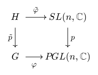
Here, $p$ is the canonical projection of $SL(n,\mathbb{C}) \to SL(n,\mathbb{C})/C_n$. It suffices to show that $\tilde\varphi$ is similar to a unitary representation. Explicitly, one has
with $\tilde\varphi:(g,A) \mapsto A$ and $\tilde{p}:(g,A) \to g$. Since $G$ is compact and $\tilde{p}$ has finite kernel $C_n$, one sees that $H$ is a compact Lie group. Therefore the matrix representation $\tilde\varphi:H \to SL(n,\mathbb{C})$ is similar to a homomorphism $H \to SU(n)$, from which the lemma follows. $\square$
Therefore we are reduced to considering homomorphisms
for sake of this post. But we are not done yet. Having to deal with a quotient group is not satisfactory anyway.
Since $SU(n)$ is simply connected (see this video), the projections $SU(n) \to SU(n)/C_n$ are universal coverings. In particular, when $n=2$, we see $SU(2) \to SU(2)/C_2 = SO(3)$ is our well-known universal covering. If we lift $\varphi$ to universal coverings, we see ourselves dealing with $SU(2) \to SU(n)$. To be precise, we have the following commutative diagram (universal cover is a functor):
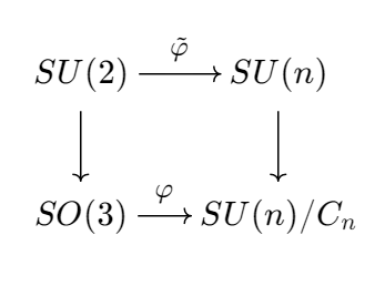
Dealing with $\tilde\varphi$ is much simpler. Physicists are more interested in unitary representations of the quaternion group $SU(2) = \operatorname{Spin}(3)$ rather than $SO(3)$, even though it looks more natural.
Now we are interested in finding all unitary representations that can be pushed down to a projective representation of $SO(3)$. We have two questions:
Question 1. Does it suffice to consider maps of the form $\tilde\varphi:SU(2)\to SU(n)$?
The answer is yes. Notice that every homomorphism $f:SU(2) \to U(1)$ has to be trivial. If not, then $\ker f$ should be a nontrivial proper normal subgroup of $SU(2)$, i.e. it has to be $C_2$. But $SU(2)/C_2 \cong SO(3)$. A contradiction.
Also recall the exact sequence
Let $g:SU(2) \to U(n)$ be any homomorphism, and consider the canonical projection $\pi:U(n) \to \frac{U(n)}{SU(n)}=U(1)$. We see $\pi \circ g$ sends any elements in $SU(2)$ to $1$, meaning the image of $SU(2)$ in $U(n)$ must bee in $SU(n)$. Therefore, by considering maps of the form $SU(2) \to SU(n)$, we are not missing anything. $\square$
Question 2. What should be considered in order to determine whether $\tilde\varphi:SU(2) \to SU(n)$ can be pushed down into a morphism $\varphi:SO(3) \to SU(n)/C_n$?
The answer is, one should consider the element $-I$. Let $p:SU(2) \to SO(3)$ be the universal covering, and let $p_n:SU(n) \to SU(n)/C_n$ be the corresponding universal covering. For $\tilde\varphi:SU(2) \to SU(n)$, we want to know when there will be a homomorphism $\varphi:SO(3) \to SU(n)/C_n$ such that $p_n \circ \tilde\varphi = \varphi \circ p$.
Notice that $p(-I)=I$, therefore, should $\varphi$ exist, one has $p_n \circ \tilde\varphi(-I)=e$, the identity in the group $SU(n)/C_n$, because one should have $\varphi(I)=e$. Hence $\tilde\varphi(-I) \in \ker p_n$. Therefore $\varphi(-I)$ can be identified as a $n$th root of unity. Since $\tilde\varphi(-I)\tilde\varphi(-I)=\tilde\varphi(I)$, we see $\tilde\varphi(-I)$ should also be identified as a square root of $1$. That is, $\tilde\varphi(-I)$ is either $\operatorname{id}$ or $-\operatorname{id}$. We discuss these two cases in the following question.
On the other hand, if $\tilde\varphi(-I)=\pm\operatorname{id}$, then one can verify that $p_n \circ \tilde\varphi \circ p^{-1}$ can be well-defined. Therefore $\tilde\varphi$ can be pushed down into a morphism of $SO(3)$ if and only if $\tilde\varphi(-I)=\pm\operatorname{id}$. $\square$
Question 3. Let $W=\bigoplus_n k_n V_n$ be a representation of $SU(2)$. What will happen if it can be pushed down to a projective representation of $SO(3)$?
Let $\tilde\varphi:SU(2) \to SU(n)$ be the homomorphism corresponding to $W$. We have known for certain that when $\tilde\varphi$ can be pushed down to $SO(3)$ if and only if $\tilde\varphi(-I)=\pm\operatorname{id}$.
If $\tilde\varphi(-I)=\operatorname{id}$, then all the $n$ have to be even because the action on the polynomials cannot be the identity when $n$ is odd. If $\tilde\varphi(-I)=-\operatorname{id}$, then all the $n$ have to be odd because when $n$ is even the action of $-I$ on the polynomials must be the identity.
To be more explicit, $W=\bigoplus_n k_{2n}V_{2n}$ or $W=\bigoplus_{n}k_{2n+1}V_{2n+1}$.
Theorem 1. The projective representations of $SO(3)$ are given up to conjugations of $SU(2)$ of the form
depending on whether $(-I)$ acts by $\operatorname{id}$ or $-\operatorname{id}$.
In brief, when thinking about projective representations of $SO(3)$, one thinks about polynomials in two variables whose terms are either all even or all odd.
When studying $\tilde\varphi:SU(2) \to SU(n)$, we see $\tilde\varphi(-I)$ can be identified both as a $n$th root of unity and a square root of unity. When $n$ is odd however, we see $\tilde\varphi(-I)$ cannot be identified as $-1$, i.e. $-I$ cannot act as $-\operatorname{id}$. Unexpectedly, number theory plays a small role here.
Let $K$ be an algebraically closed field of characteristic $0$. Instead of studying the polynomial ring $K[X]$ as a whole, we pay a little more attention to each polynomial. A reasonable thing to do is to count the number of distinct zeros. We define
For example, If $f(X)=(X-1)^{100}$, we have $n_0(f)=1$. It seems we are diving into calculus but actually there is still a lot of algebra.
Theorem 1 (Mason-Stothers). Let $a(X),b(X),c(X) \in K[X]$ be polynomials such that $(a,b,c)=1$ and $a+b=c$. Then
Proof. Putting $f=a/c$ and $g=b/c$, we have
This implies
We interrupt the proof here for some good reasons. Rational functions of the form $f’/f$ remind us of the chain rule applied to $\log{x}$. In the context of calculus, we have $\left(\log{f(x)}\right)’=f’/f$. On the ring $K[x]$, we define $D:K[x] \to K[x]$ to be the formal derivative morphism. Then this endomorphism extends to $K(x)$ by
On $K(x)^\ast$ (read: the multiplicative group of the rational function field $K(x)$), we define the logarithm derivative
It follows that
Also observe that, just as in calculus, if $f$ is a constant function, then $D(f)=0$. Now we write
Then it follows that
Now we can be back to the proof.
Proof (continued). Since $K$ is algebraically closed,
We see, for example
Therefore
Likewise
Combining both, we obtain
Next, multiplying $f’/f$ and $g’/g$ by
which has degree $n_0(abc)$ (since $(a,b,c)=1$, these three polynomials share no root). Both $N_0f’/f$ and $N_0g’/g$ are polynomials of degrees at most $n_0(abc)-1$ (this is because $\deg h’=\deg h-1$ for non-constant $h \in K[X]$, while $f$ and $g$ are non-constant (why?); we assume $\operatorname{char} K=0$ for this reason).
Next we observe the degrees of $a,b$ and $c$. Since $a+b=c$, we actually have $\deg c \le \max\{\deg a,\deg b\}$. Therefore $\max\{\deg a,\deg b,\deg c\}=\max\{\deg a,\deg b\}$. From the relation
and the assumption that $(a,b)=1$, one can find polynomial $h \in K[X]$ such that
Taking the degrees of both sides, we see
This proves the theorem. $\square$
We present some applications of this theorem.
Corollary 1 (Fermat’s theorem for polynomials). Let $a(X),b(X)$ and $c(X)$ be relatively prime polynomials in $K[X]$ such that not all of them are constant, and such that
Then $n \le 2$.
Alternatively one can argue the curve $x^n+y^n=1$ on $K(X)$.
Proof. Since $a,b$ and $c$ are relatively prime, we also have $a^n$, $b^n$ and $c^n$ to be relatively prime. By Mason-Stothers theorem,
Replacing $a$ by $b$ and $c$, we see
It follows that
In this case $n<3$. $\square$
Corollary 2 (Davenport’s inequality). Let $f,g \in K[X]$ be non-constant polynomials such that $f^3-g^2 \ne 0$. Then
One may discuss cases separately on whether $f$ and $g$ are coprime, and try to apply Mason-Stothers theorem respectively, and many documents only record the proof of coprime case, which is a shame. The case when $f$ and $g$ are not coprime can be a nightmare. Instead, for sake of accessibility, we offer the elegant proof given by Stothers, starting with a lemma about the degree of the difference of two polynomials.
Lemma 1. Suppose $p,q \in K[X]$ are two distinct non-constant polynomials, then
Proof. Let $k(f)$ be the leading coefficient of a polynomial $f$. If $\deg p \ne \deg q$ or $k(p) \ne k(q)$, then $\deg(p-q)\ge \deg p \ge \deg p - n_0(p)-n_0(q)+1$ because $n_0(p) \ge 1$ and $n_0(q) \ge 1$.
Next suppose $\deg p = \deg q$ and $k(p)=k(q)$. If $(p,q)=1$, then by Mason-Stothers,
Otherwise, suppose $(p,q)=r$. Then $p/r$ and $q/r$ are coprime. Again by Mason-Stothers,
Therefore
On the other hand,
Combining all these inequalities, we obtain what we want. $\square$
Proof (of corollary 2). Put $\deg{f}=m$ and $\deg{g}=n$. If $3m \ne 2n$, then
because $m \ge 1$. Next we assume that $3m=2n$, or in other word, $m=2r$ and $n=3r$. By lemma 1, we can write
This proves the inequality. $\square$
One may also generalise the case to $f^m-g^n$. But we put down some more important remarks. First of all, Mason-Stothers is originally a generalisation of Davenport’s inequality (by Stothers). I personally do not think any mortal can find the original paper of Davenport’s inequality, but on [Shioda 04] there is a reproduced proof using linear algebra (lemma 3.1).
For more geometrical interpretation, one may be interested in [Zannier 95], where Riemann’s existence theorem is also discussed.
In Stothers’s paper [Stothers 81], the author discussed the condition where the equality holds. If you look carefully you will realise his theorem 1.1 is exactly the Mason-Stothers theorem.
Definition. For a polynomial with coefficients in a number field $K$
the height of $f$ is defined to be
where
is the Gauss norm for any place $v$.
Here, $M_K$ refers to the canonical set of non-equivalent places on $K$. See first four pages of this document for a reference.
As one can expect, this can tell us about some complexity of a polynomial, just like how the height of an algebraic number tells us its complexity. Let us compute some examples.
Let us consider the simplest one
first. Since $|x^2-1|_v=1$ for all places $v$, the height of $f$ is a sum of $0$, which is still $0$.
Next, we take care of a polynomial that involves prime numbers
We see $|g(x)|_\infty=2$, $|g(x)|_2=2^{-(-2)}=4$, $|g(x)|_3=3^{-(-1)}=3$, and the Gauss norm is $1$ for all other primes. Therefore
Put $u(x,y)=\sqrt{2}x^2 + 3\sqrt{2}xy+5y^2+7 \in \mathbb{Q}(\sqrt{2})[x,y]$, we can compute its height carefully. Notice that $|\sqrt{2}|_v=\sqrt{|2|_v}$ for all places $v$ and we therefore have
If $f \in K[s_1,\dots,s_n]$ and $g \in K[t_1,\dots,t_m]$ are two polynomials in different variables, then as a polynomial in $K[s_1,\dots,s_n;t_1,\dots,t_m]$, $fg$ has height $h(f)+h(g)$. This is immediately realised once we notice that the height of a polynomial is equal to the height of the vector of coefficients in appropriate projective space. The identity $h(fg)=h(f)+h(g)$ follows from the Segre embedding.
But if variables coincide, things get different. For example, $h(x+1)=0$ but $h((x+1)^2)=2$. This is because we do not have $|fg|_\infty=|f|_\infty|g|_\infty$. Nevertheless, for non-Archimedean places, things are easier.
Gauss’s lemma. If $v$ is not Archimedean, then $|fg|_v=|f|_v|g|_v$.
Proof. First of all, it suffices to prove it for univariable cases. If $f$ and $g$ have multiple variables $x_1,\dots,x_n$, let $d$ be an integer greater than the degree of $fg$. Then the Kronecker substitution
reduces our study into $K[t]$. This is because, with such a $d$, this substitution gives a univariable polynomial with the same set of coefficients.
Therefore we only need to show that $|f(t)g(t)|_v=|f(t)|_v|g(t)|_v$. Without loss of generality we assume that $|f(t)|_v=|g(t)|_v=1$. Write $f(t)=\sum a_k t^k$ and $g(t)=\sum b_k t^k$, we have $f(t)g(t)=\sum c_jt^j$ where $c_j=\sum_{j=k+l}a_kb_l$.
We suppose that $|fg|_v<1$, i.e., $|c_j|_v<1$ for all $j$, and see what contradiction we will get. If $|a_j|=1$ for all $j$, then $|c_j|_v<1$ implies that $|b_k|_v<1$ for all $k$ and therefore $|g|_v<1$, a contradiction. Therefore we may assume that, without loss of generality, $|a_0|_v<1$ but $|a_1|_v=1$. Then, since
we have $|a_1b_{j-1}|_v=|b_{j-1}|_v<1$ for all $j \ge 1$. It follows that $|g(t)|_v<1$, still a contradiction. $\square$
So much for non-Archimedean case. For Archimedean case things are more complicated so we do not have enough space to cover that. Nevertheless, we have
Gelfond’s lemma. Let $f_1,\dots,f_m$ be complex polynomials in $n$ variables an set $f=f_1\cdots f_n$, then
where $d$ is the sum of the partial degrees of $f$, and $\ell_\infty(f)=\max_j|a_j|=|f|_\infty$.
Combining Gelfond’s lemma and Gauss’s lemma, we obtain
Is not actually given by Mahler initially. It was named after Mahler because he successfully extended it to multivariable cases in an elegant way. We will cover the original motivation anyway.
Say we want to find prime numbers large enough. Pierce came up with an idea. Consider $p(x) \in \mathbb{Z}[x]$, which is factored into
Consider $\Delta_n=\prod_i(\alpha^n_i-1)$. Then by some Galois theory, this is indeed an integer. So perhaps we may find some interesting integers in the factors of $\Delta_n$. Also, we expect it to grow slowly. Lehmer studied $\frac{\Delta_{n+1}}{\Delta_n}$ and observed that
So it makes sense to compare all roots of $p(x)$ with $1$. He therefore suggested the following function related to $p(x)$:
This number appears if we consider $\lim_{n \to \infty}\Delta_{n+1}/\Delta_n$.
He also asked the following question, which is now understood as Lehmer conjecture, although in his paper he addressed it as a problem instead of a conjecture:
Is there a constant $c$ such that, $M(p)>1 \implies M(p)>c$?
It remains open but we can mention some key bounds.
and actually this is the finest result that has ever been discovered. It was because of this discovery that he gave his problem.
This polynomial has also led to the discovery of a large prime number $\sqrt{\Delta_{379}}=1, 794, 327, 140, 357$, although by studying $x^3-x-1$, we have found a bigger prime number $\Delta_{127}=3, 233, 514, 251, 032, 733$.
for some $c>0$.
Definition. For $f \in \mathbb{C}[x_1,\dots,x_n]$, the Mahler measure is defined to be
where $d\mu_i=\frac{1}{2\pi}d\theta_i$, i.e., $d\mu_1\dots d\mu_n$ corresponds to the (completion of) Harr measure on $\mathbb{T}^n$ with total measure $1$.
We see through Jensen’s formula that when $n=1$ this coincides with what we have defined before. Observe first that $M(fg)=M(f)M(g)$. Consider $f(t)=a\prod_{i=1}^{d}(t-\alpha_i)$, then
On the other hand, as an exercise in complex analysis, one can show that
Combining them, we see
Taking the logarithm we also obtain Jensen’s formula
We first give a reasonable and useful estimation of $M(f)$, which will be used to prove the Northcott’s theorem.
Definition. For $f(t)=a_dt^d+\dots+a_0$, the $\ell_p$-norm of $f$ is naturally defined to be
For $p=\infty$, we have $\ell_\infty(f)=\max_j|a_j|$.
Lemma 1. Notation being above, $M(f) \le \ell_1(f)$ and
Proof. To begin with, we observe those obvious ones. First of all,
Therefore
Next, by Jensen’s inequality
However, by Parseval’s formula, the last term equals
For the remaining inequality, we use Vieta’s formula
and therefore
for all $0 \le r \le d$. Replacing $|a_{d-r}|$ with $\ell_\infty(f)$, we have finished the proof. $\square$
Before proving Northcott’s theorem, we show the connection between Mahler measure and heights.
Proposition 1. Let $\alpha \in \overline{\mathbb{Q}}$ and let $f$ be the minimal polynomial of $\alpha$ over $\mathbb{Z}$. Then
and
Proof. Put $d=\deg(\alpha)$ and write
Choose a number field $K$ that contains $\alpha$ and is a Galois extension of $\mathbb{Q}$, with Galois group $G$. Then $(\sigma\alpha:\sigma \in G)$ contains every conjugate of $\alpha$ exactly $[K:\mathbb{Q}]/d$ times. Since $a_0,\dots,a_d$ are coprime, for any non-Archimedean absolute value $v \in M_K$, we must have $\max_i|a_i|_v=|f|_v=1$. Combining with Gauss’s lemma and Galois theory, we see
Now we are ready to compute the height of $\alpha$ to rediscover the Mahler’s measure. Notice that
We therefore obtain
The last term corresponds to what we have computed above about non-Archimedean absolute values so we break it down a little bit:
for some $u \mid \infty$, according to the product formula. On the other hand, for $v \mid \infty$,
All in all,
The second assertion follows immediately because
The set of non-zero algebraic integers of height $0$ lies on the unit circle, and they are actually roots of unit, by Kronecker’s theorem. However keep in mind that algebraic integers on the unit circle are not necessarily roots of units. See this short paper.
When it comes to algebraic integers of small heights, things may get complicated, but Northcott’s theorem assures that we will be studying a finite set.
Northcott’s Theorem. Given an integer $N>0$ and a real number $H \ge1$, there are only a finite number of algebraic integers $\alpha$ satisfying $\deg(\alpha) \le N$ and $h(\alpha) \le \log H$.
Proof. Let $\alpha$ be a algebraic integer of degree $d<N$ and height $h(\alpha) \le \log H$. Suppose $f(t)=a_dt^d+\dots+a_0 \in \mathbb{Z}[t]$ is the minimal polynomial of $\alpha$. Then lemma 1 shows us that
On the other hand, by proposition 1,
we have actually
This gives rise to no more than $(2\lfloor (2H)^d \rfloor+1)^{d+1}$ distinct polynomials $f$, which produces at most $d(2\lfloor (2H)^d \rfloor+1)^{d+1}<\infty$ algebraic integers. Ranging through all $d \le N$ we get what we want. $\square$
We also have the Northcott property, where we do not care about degrees. A set $L$ of algebraic integers is said to satisfy Northcott property if, for every $T>0$, the set
is finite. Such a set $L$ is said to satisfy Bogomolov property if, there exists $T>0$ such that the set
is empty. As a matter of elementary topology, Northcott property implies Bogomolov property. It would be quite interesting if $L$ is a field. This paper can be quite interesting.
Erico Bombieri, Walter Gubler, Heights in Diophantine Geometry.
Michel Waldschmidt, Diophantine Approximation on Linear Algebraic Groups, Transcendence Properties of the Exponential Function in Several Variables.
Chris Smyth, THE MAHLER MEASURE OF ALGEBRAIC NUMBERS: A SURVEY.
Let $F$ be a non-Archimedean local field, meaning that $F$ is complete under the metric induced by a non-Archimedean absolute value $|\cdot|$. Consider the ring of integers
and its unique prime (hence maximal) ideal
The residue field $k=\mathfrak{o}_F/\mathfrak{p}$ is finite because it is compact and discrete. For compactness notice that $\mathfrak{o}_F$ is compact, and the canonical projection $\mathfrak{o}_F \to k$ is open. For discreteness, notice that $\mathfrak{p}$ is open, connected and contains the unit.
Let $f \in \mathfrak{o}_F[x]$ be a polynomial. Hensel’s lemma states that, if $\overline{f} \in k[x]$, the reduction of $f$, has a simple root $a$ in $k$, then the root can be lifted to a root of $f$ in $\mathfrak{o}_F$ and hence $F$. This blog post is intended to offer a well-organised proof of this lemma.
To do this, we need to use Newton’s method of approximating roots of $f(x)=0$, something like
We know that $a_n \to \zeta$ where $f(\zeta)=0$ at a $A^{2^n}$ speed for some constant $A$, in calculus (do Walter Rudin’s exercise 5.25 of Principles of Mathematical Analysis if you are not familiar with it, I heartily recommend.). Now we will steal Newton’s method into number theory to find roots in a non-Archimedean field, which is violently different from $\mathbb{R}$, the playground of elementary calculus.
We will also use induction, in the form of which I would like to call “double induction”. Instead of claiming that $P(n)$ is true for all $n$, we claim that $P(n)$ and $Q(n)$ are true for all $n$. When proving $P(n+1)$, we may use $Q(n)$, and vice versa.
This method is inspired by this lecture note, where actually a “quadra induction” is used, and everything is proved altogether. Nevertheless, I would like to argue that, the quadra induction is too dense to expose the motivation and intuition of this proof. Therefore, we reduce the induction into two arguments and derive the rest with more reasonings.
Hensel’s Lemma. Let $F$ be a non-Archimedean local field with ring of integers $\mathfrak{o}_F=\{\alpha \in F:|\alpha| \le 1\}$ and prime ideal $\mathfrak{p}=\{\alpha \in F:|\alpha|<1\}$. Let $f \in \mathfrak{o}_F[x]$ be a polynomial whose reduction $\overline{f} \in k[x]$ has a simple root $a \in k$, then $a$ can be lifted to $\alpha \equiv a \mod \mathfrak{p}$, such that $f(\alpha)=0$.
By simple root we mean $\overline{f}(a)=0$ but $\overline{f}’(a) \ne 0$. Before we prove this lemma, we see some examples.
Put $F=\mathbb{Q}_7$. Then $\mathfrak{o}_F=\mathbb{Z}_7$, $\mathfrak{p}=7\mathbb{Z}_7$ and $k=\mathbb{F}_7$. We show that square roots of $2$ are in $F$. Note $\overline{f}(x)=x^2-2=(x-3)(x+3) \in k[x]$, we therefore two simple roots of $\overline{f}$, namely $3$ and $-3$. Lifting to $\mathfrak{o}_F$, we have two roots $\alpha_1 \equiv 3 \mod 7\mathbb{Z}_7$ and $\alpha_2 \equiv -3 \mod 7\mathbb{Z}_7$, of $f$. For $\alpha_1$, we have
Hence we can put $\alpha=\sqrt{2}=3+7+2\cdot 7^2+6\cdot 7^3\cdots\in\mathbb{Z}_7 \subset \mathbb{Q}_7$. Likewise $\alpha_2$ can be understood as $-\sqrt{2}$. This expansion is totally different from our understanding in $\mathbb{Q}$ or $\mathbb{R}$.
Since $k$ is a finite field, we see $k^\times$ is a cyclic group of order $q-1$ where $q=p^n=|k|$ for some prime $p$. It follows that $x^{q-1}=1$ for all $x \in k^\times$. Therefore $f(x)=x^{q-1}-1$ has $q-1$ distinct roots in $k$. By Hensel’s lemma, $F$ contains all $(q-1)$st roots of unity. It does not matter whether $F$ is isomorphic to $\mathbb{Q}_p$ or $\mathbb{F}_q((t))$.
Pick any $a_0 \in \mathfrak{o}_F$ that is a lift of $a\mod\mathfrak{p}$. Define
then we claim that $a_n$ converges to the root we are looking for.
First of all, we need to show that $a_n \in \mathfrak{o}_F$, i.e., $|a_n| \le 1$ for all $n$. It suffices to show that $|f(a_{n-1})/f’(a_{n-1})| \le 1$. We firstly observe the case when $n=1$.
Since $\overline{f}(a)=0$ but $\overline{f}’(a) \ne 0$, we have $f(a_0) \in \mathfrak{p}$ but $f’(a_0)\not\in\mathfrak{p}$. As a result, $|f(a_0)|<1$ but $|f’(a_0)|=1$. As a result, $|f(a_0)/f’(a_0)|<1$, which implies that $f(a_0)/f’(a_0) \in \mathfrak{o}_F$ and therefore $a_1 \in \mathfrak{o}_F$.
By Taylor’s theorem.
for some $g_n \in \mathfrak{o}_F[x]$. When $n=1$, we see $g_1(a_1) \in \mathfrak{o}_F$ and as a result $|g_1(a_1)| \le 1$. Therefore
Since $a_1 \in \mathfrak{o}_F$, we also see that $f(a_1) \in \mathfrak{o}_F$ hence its absolute value is not greater than $1$. As a result $|f(a_1)/f’(a_1)| \le 1$, which implies that $a_2 \in \mathfrak{o}_F$.
This inspires us to claim the following two statements:
(a) $|f(a_n)| < 1$ for all $n \ge 0$.
(b) $|f’(a_n)|=|f’(a_0)|=1$ for all $n \ge 0$.
We have verified (a) and (b) for $n=0$ and $n=1$. Now assume that (a) and (b) are true for $n-1$, then, for $n$, we will verify as follows.
First of all, by (a) and (b) for $n-1$, we see $a_n \in \mathfrak{o}_F$.
Consider the Taylor’s expansion
where $h_n \in \mathfrak{o}_F[x]$. It follows that $|h_n(a_n)| \le 1$. Since $|f’(a_{n-1})|=1$, by (b) we actually have
To prove (b) for $n$, we consider the Taylor’s expansion
Notice that since $a_n \in \mathfrak{o}_F$, we have $f’’(a_{n-1}),g_n(a_n) \in \mathfrak{o}_F$. By (a) and (b) for $n-1$, we see
Hence
bearing in mind that for a non-Archimedean absolute value, $|x+y|=\max\{|x|,|y|\}$ iff $|x| \ne |y|$. Through this process we have also proved (b).
We need to show that $\{a_n\}$ is a Cauchy sequence. To do this, it suffices to show that $|f(a_n)| \to 0$ sufficiently quick. Recall in the proof of (a) we have shown that $|f(a_n)| \le |f(a_{n-1})|^2$ for all $n$. By applying this relation inductively, we see $|f(a_n)| \le |f(a_0)|^{2^n}$. Since $|f(a_0)|<1$, it follows that $|f(a_n)| \to 0$ as $n \to \infty$.
For any $\varepsilon>0$, there exists $N>0$ such that $|f(a_n)| <\varepsilon$ for all $n \ge N$. As a result, for all $m>n>N$, we have
Therefore $\{a_n\}$ is Cauchy. Since $F$ is complete, $a_n$ converges to some $\alpha \in \mathfrak{o}_F \subset F$ such that $f(\alpha)=\lim_{n \to \infty}f(a_n)=0$.
In local fields, congruence is determined by inequality. In fact, we only need to show that $|\alpha-a_0|<1$, which means that $\alpha-a_0 \in \mathfrak{p}$, and therefore $\alpha \equiv a \mod \mathfrak{p}$ as expected. To do this, we show by induction that $|a_n-a_0|<1$. For $n=1$ we see $|a_1-a_0|=|f_0|<1$.
Suppose $|a_{n-1}-a_0|<1$ then
Therefore $|\alpha-a_0|=\lim_{n \to \infty}|a_n-a_0|<1$, from which the result follows. $\square$
In fact we have not explicitly used the fact that $a$ is a simple root. We only used the fact that $|f(a_0)|<1$ but $|f’(a_0)|=1$. Moreover, what really matters here is that $|f(a_n)|$ converges to $0$ quick enough. Therefore $1$ may be replaced by a smaller constant. For this reason we introduce a stronger version of Hensel’s lemma.
Hensel’s lemma, stronger version. Let $F$ be a non-Archimedean local field with ring of integers $\mathfrak{o}_F$. Suppose there exists $a \in \mathfrak{o}_F$ such that $|f(a)|<|f’(a)|^2$, then there exists some $b \in \mathfrak{o}_F$ such that $f(b)=0$ and $|b-a|<|f’(a)|$.
Instead of asserting $|f’(a_n)|=1$ for all $n$, we claim that $|f’(a_n)|=|f’(a_0)|$ (as it should be!). Instead of asserting $|f(a_n)|<1$, we claim that $|f(a_n)| \le \lambda^{2^n}|f’(a_0)|$ where $\lambda=|f(a_0)|/|f’(a_0)|^2$. The proof will be nearly the same.
For example, we can find a square root of $257$ in $\mathbb{Z}_2 \subset \mathbb{Q}_2$. The polynomial $f(x)=x^2-257$ is reduced to $\overline{f}(x)=x^2-1=(x-1)^2$ in $\mathbb{F}_2[x]$, where $1$ is not a simple root. Therefore we cannot apply the original version of Hensel’s lemma to this polynomial. Nevertheless, we see $f(1)=-256$ and $f’(1)=2$. Therefore $|f(1)|=\frac{1}{2^8}$ while $|f’(1)|=\frac{1}{2}$. We can apply Newton’s method here to find a square root of $257$ without worrying about repeated roots.
There are a lot of variants of Hensel’s lemma, for example you can do exercise 10.9 of Atiyah-MacDonald. In fact, we later even have Henselian ring and Henselisation of a ring.
There are some other proofs of Hensel’s lemma in this post, for example, since Newton’s method can also be understood as a contraction mapping, we can also prove it using properties of contraction mapping (see K. Conrad’s note).
Representation theory is important in various branches of mathematics and physics. When studying representation of finite groups, we have quite some algebra and combinatorics. When differentiation (more precisely, smoothness) joins the party, we have Lie group, involving calculus, linear algebra, geometry and much more. Especially, theories around $SU(2)$ and $SO(3)$ are of great importance. On one hand, they are those simplest non-elementary and high-dimensional Lie groups. On the other hand, they describes rotations in $\mathbb{C}^2$ and $\mathbb{R}^3$ respectively, which is “physically realistic”. I believe students in physics have more to say.
In this post we develop a way to study irreducible representations of these two Lie groups, in a mathematician’s way. I try my best to make sure that everything is down-to-earth, and everything can be “reduced” to 19th (pre-modern) mathematics.
Nevertheless, the reader has to be assumed to be familiar with elementary languages of representation theory (and you know that, there are a lot of abuse of language), which I think is not a problem because otherwise you wouldn’t be reading this post. You need to recall eigenvalue theories in linear algebra, as well as Fourier series. We need the fact that the trigonometric system is complete. In other words trigonometric polynomials are dense in the space of continuous functions. $\def\sym{\operatorname{Sym}}$
We will first study $SU(2)$ and a first classification of irreducible representations of $SO(3)$ follows at once. This is because we have an isomorphism
This is to say, $SU(2)$ is a “double cover” of $SO(3)$. To see this, notice that $SU(2) \cong S^3$ and $SO(3) \cong \mathbb{R}P^3$ as Lie groups, meanwhile $\mathbb{R}P^3 \cong S^3/\{-1,1\}$ can be considered as the definition.
Of course, by representation we mean finite dimensional and unitary representations.
Indeed it seems we have nowhere to start. Instead of trying to find all of them, we will try to work on seemingly immediate representations and it turns out that they are all we are looking for.
Let $V_0$ be the trivial representation on $\mathbb{C}$ and $V_1$ be the standard representation on $\mathbb{C}^2$, which is given by ordinary matrix multiplication. These representations are irreducible. We want to extend this family to $V_n$ for $n \ge 2$. It is natural to think about generate representations of higher dimensions through $V_1$. Here are several ways available.
Direct sum: $\bigoplus_{i=1}^{n}V_1$. The dimension is $2n$ and unfortunately, the representation is determined by each component so essentially there is no “new thing”.
Tensor product: $\bigotimes_{i=1}^{n}V_1$. The dimension is $2^n$ which is way too big.
Wedge product: $\bigwedge^{n}V_1$. It stops at $n=2$ and we have to deal with $u \wedge v = - v \wedge u$. This can be annoying.
Symmetric product: $\sym^{n}V_1$. The dimension is $n+1$ and it doesn’t stop. Besides, it can be understood as homogeneous polynomials of degree $n$ in two variables. This is a fantastic choice. Besides we have $\sym^0 V_1=V_0$ so nothing is abruptly excluded.
Put $V_n=\sym^nV_1$, which can be understood as the space of homogeneous polynomials of degree $n$ in variables $z_1$ and $z_2$. $V_n$ therefore has a canonical basis
And we will make use of it later.
For each $g \in SU(2)$, we have a left action
In other words, $\rho(g)P(z)=P(zg)$ where $z=(z_1,z_2)$ and $zg$ is matrix multiplication. Each $g \in SU(2)$ has matrix representation
Then
When there is no confusion, we will write $gP(z)=P(zg)$, viewing $g$ itself as an automorphism of $V_n$. One can also replace $SU(2)$ with $GL(2,\mathbb{C})$ but we are not studying that bigger one.
Since $z \mapsto zg$ is a homogeneous map of degree $1$ as it is linear and is non-degenerate, we have $gP(z) \in V_n$. In other words, $V_n$ are $SU(2)$-invariant. We now have a well-defined representation. Note $V_0=\mathbb{C}$ so the representation is trivial, and $V_1=\mathbb{C}^2$ yields linear maps. Again, nothing is abruptly excluded. Even more satisfyingly, those $V_n$ are all irreducible.
Proposition 1. The representations $V_n$ are irreducible.
Proof. By Schur’s lemma, we need to show that each $SU(2)$-equivariant automorphism $A$ of $V_n$ is a non-zero multiple of the identity, i.e. $A=\lambda I$ for some $\lambda \ne 0$. By definition, for each $g \in SU(2)$, we have $A\rho(g)P=\rho(g)AP$ for all $P \in V_n$. And for simplicity we write $Ag=gA$, realising $g$ as a linear transform of $V_n$, instead of an element of $SU(2)$.
The group $SU(2)$ can be complicated, but $U(1) \cong S^1$ is simple and can be considered as a subgroup of $SU(2)$ in two ways. We show that these two ways are just enough to expose the irreducibility of $V_n$.
First of all we embed $S^1$ into $SU(2)$ by
Call the matrix right hand side $g_a$. Then
for all $k$. This is to say, $P_k$ is the eigenvector corresponding to eigenvalue $a^{2k-n}$. As $g_aA=Ag_a$, information on eigenvalues and eigenvectors can help a lot so we dig into it first.
Since $\{P_k\}$ are linearly independent, under this basis, we have a matrix representation
but we don’t know how eigenspaces are spanned because we may have $a^j=a^k$ for $j \ne k$. However, the number $a$ can always be chosen that $a^{-n},a^{-n+2},\dots,a^n$ are pairwise distinct (for example, one can pick $a$ to be a primitive $m$-th root of $1$ and $m$ is big enough). As a result, $g_a$ has $n$ distinct eigenvalues. Therefore, the $a^{2k-n}$-eigenspace can only be generated by $P_k$.
On the other hand, by definition of $A$, we have
Hence $AP_k$ lies in $a^{2k-n}$-eigenspace. Therefore we have $AP_k=c_kP_k$ for some $c_k \ne 0$. In other words, $P_k$ is the $c_k$-eigenvector of $A$. We obtain another matrix representation under the basis $\{P_k\}$
We want this matrix to be a scalar matrix. The result follows from another embedding of $U(1)$ into $SU(2)$. Note $a \in S^1$ can be determined by $t \in [0,2\pi)$, and we therefore have a matrix
Still we have $Ag_t=g_tA$. As we can see,
This follows from our observation on eigenvalues. Next, we immediately use the eigenvalue $c_n$ to obtain
This is the definition of $g_tP_n$. Comparing coefficients of $P_k$, we must have $c_k=c_n$ for all $0 \le k \le n$. Recall that $\{P_k\}$ is a basis so coefficients must be unique for a given vector. But we have already obtained what we want: $A=c_n I$. $\square$
So far we have used diagonalisation of representations of $SU(2)$ but the diagonalisation of $SU(2)$ itself is not touched yet. Neither have we made use of character functions. So now we invite them to the party.
Let’s recall diagonalisation in $SU(2)$. Pick $g \in SU(2)$. First of all it is diagonalisable. Let $\lambda_1$ and $\lambda_2$ be their two eigenvalues, then $|g|=\lambda_1\lambda_2=1$. Therefore we have
where $\lambda$ is one of the eigenvalues of $g$. Since the diagonalised matrix is still in $SU(2)$, we have $|\lambda|=1$, i.e., $\lambda \in S^1$. We therefore write $g \sim e(t) \sim e(-t)$ where
We see, $e(s) \sim e(t)$ if and only if $s = \pm t \mod 2\pi$. By periodicity of $\exp$ function, we also see $e(t)$ is in particular $2\pi$-periodic. If $f:SU(2) \to \mathbb{C}$ is a class function, then $f \circ e:\mathbb{R} \to \mathbb{C}$ is an even $2\pi$-periodic function. Conversely, given an even $2\pi$-periodic function $h:\mathbb{R} \to \mathbb{C}$, we can recover it as a class function, and the process is as follows.
Define $\Lambda:SU(2) \to S^1$ sending $g \in SU(2)$ to the eigenvalue of $g$ with non-negative imaginary part (one can also pick non-positive one, because $h$ is even). Then $E:SU(2) \to [0,\pi]$ given by $g \mapsto \frac{1}{i}\log\Lambda(g)$ is a well defined function sending $g$ into $\mathbb{R}$ and $h \circ E:SU(2) \to \mathbb{C}$ is a class function. Besides we have $E \circ e(t)= \pm t \mod 2\pi$ and $e \circ E(g)$ is the diagonalisation of $g$. Therefore $h \circ E \circ e(t)=h(t)$ and $f \circ e \circ E(g)=f$ as is expected.
With help of this $e(t)$ and $E(t)$, we have this correspondence
Recall that the space on the right hand side has a countable uniform basis
In other words, $\{\cos{nt}\}_{n \ge 0}$ spans a dense subspace. This is about the completeness of trigonometric system. Since there are only even functions, $\sin{nt}$ are excluded. For a reference to the completeness, one can check 4.25 Real and Complex Analysis by W. Rudin.
For class functions, we certainly want to know about characters. Let $\chi_n$ be the character of $V_n$, then
When $t \in \pi\mathbb{Z}$, then $\chi_n(e(t)) \in \mathbb{Z}$. Otherwise, as a classic exercise in calculus, we have
We have $\kappa_0(t)=1$. For $\kappa_n(t)$ when $n >0$, we have
We see $\kappa_1(t)=2\cos{t}$. By induction, every $\kappa_n(t)$ is a polynomial in variables $1,\cos{t},\dots,\cos{nt}$. Therefore $\{\kappa_n(t)\}_{n \ge 0}$ spans the same space as $\{\cos{nt}\}_{n \ge 0}$, which is dense in the space of even $2\pi$-periodic functions. Note the $\kappa_n(t)$ are linearly independent, because the leading term is $\cos{nt}$.
The argument above shows that $\chi_n$ spans a dense subspace in the space of class functions. In other word, $\chi_n$ is the Fourier basis of class functions. As we all know, Fourier series is powerful. Let’s see how powerful it is in the calculus of Lie group $SU(2)$ itself.
Proposition 2. For continuous class function $f:SU(2) \to \mathbb{C}$, we have
Proof. On one hand, since the $V_n$ are irreducible, by fixed point theorem of representations,
Here, for a group $G$ and a representation $V$, $V^G$ is the fixed point set, i.e. the space of elements that are fixed by the action of $G$ on $V$. Since $\chi_n$ is irreducible, fixed points can only be $0$ unless the representation itself is trivial. Now we move on and check the right hand side.
On the right hand side we are looking for even $2\pi$-periodic continuous functions, reflecting the denseness of $\kappa_n(t)$. However we have $\int_{-\pi}^{\pi}\kappa_1(t)dt=\pi$ so it does not vanish on $n>0$. However, if we multiply it by $\sin^2{t}$, then it is transformed into the form $\sin{mt}\sin{nt}$ and we are familiar with this orthonormality. More precisely,
Since the functional $h \mapsto \frac{1}{2\pi}\int_{-\pi}^{\pi}h\sin^2{t}dt$ is continuous in the uniform topology and $\kappa_n$ spans a dense subspace, the result is now obtained. $\square$
Finally, surprisingly and satisfyingly enough, the denseness have actually axed out all other possibilities of irreducible representation. In other words, our search in symmetric products is optimal. We can see this through Parseval’s identity. This is the heart of this blog post.
Proposition 3. Every irreducible representation of $SU(2)$ is isomorphic to one of the $V_n$.
Proof. Suppose we have a character that is different from all of the $\chi_n$. Then the orthonormality shows that $\langle \chi,\chi_n \rangle = 0$ for all $n \ge 0$ and $\langle \chi,\chi \rangle=1$. Now let’s see why this is absurd.
Since $\{\chi_n\}_{n \ge 0}$ spans a dense subspace in the space of class functions, we actually have
Therefore
and
It is impossible to have the sum of $0$ to be $1$. $\square$
Now we head to $SO(3)$. In fact the result follows immediately from the surjection
We have $\ker\pi=\{-I,I\}$. Let $W$ be a representation of $SO(3)$, i.e., we have a map
Then
by $g \mapsto \rho(\pi(g))$ is an induced representation, and we write $\pi^\ast W$. If $W$ is irreducible, then $\pi^\ast W$ is also irreducible. In particular, $\pi^\ast\rho(-I)=\operatorname{id}_W$.
On the other hand, if $\vartheta:SU(2) \to GL(V)$ is an irreducible representation where $\vartheta(-I)=\operatorname{id}_V$, then we have an associated representation
given by $g\ker\pi \mapsto \vartheta(g)$. Let’s denote it by $\pi_\ast V$. Again, if $V$ is irreducible, then $\pi_\ast V$ is irreducible.
Therefore we have realised a correspondence
So it remains to determine those of $SU(2)$. Let $\rho_n:SU(2) \to GL(V_n)$ be an irreducible representation, then
because $P \in \mathbb{C}[z_1,z_2]$ is homogeneous of degree $n$. Therefore $-I$ acts as an identity if and only if $n$ is even. We obtain
Proposition 4. Every irreducible representation of $SO(3)$ is of the form
where $V_{2n}$ is described in proposition 2.
This is, of course, just a first classification. But to introduce a classification as explicit as what we have done for $SU(2)$, there has to be another post. As a quick overview, here is the result.
Let $P_{\ell}$ be the complex vector space of homogeneous polynomials in three variables of degree $\ell$, which can be considered as functions on $\mathbb{R}^3$ immediately. This setting makes sense immediately, just as what we have done for $SU(2)$. Then, in fact,
This is to say, $W_\ell$ can be understood as harmonic homogeneous polynomials in $\mathbb{R}^3$, which can also be considered to be uniquely determined on the unit sphere $S^2$.
In the previous post we are convinced that the Galois group of a separable irreducible polynomial $f$ can be realised as a subgroup of the symmetric group, the elements of which permute the roots of $f$. We worked on cubic polynomials over a field with characteristic not equal to $2$ and $3$, and this definitely works with $\mathbb{Q}$. In this post we go one step further.
Let $f \in \mathbb{Q}[X]$ be an irreducible polynomial of prime degree $p$. Since it is also separable (see lemma 9.12.1 on the stack project), we can safely work on its Galois group $G$. One immediately wants to question the position of $\mathfrak{S}_p$. Indeed we have $G \subset \mathfrak{S}_p$. The question is, when does the equality hold? It is not likely to have an immediate answer. However, we have some interesting sufficient conditions, which will be discussed in this post.
We present some handy results in finite group theory that will be used in the main result. One may skip this section until needed. I will collapse the proof in case one wants to treat it as an exercise.
Lemma 1. Let $p$ be a prime number. The symmetric group $\mathfrak{S}_p$ is generated by $[12 \cdots p]$ and an arbitrary transposition $[rs]$.
Proof. We prove this by presenting several sets of generators of $\mathfrak{S}_n$ where $n$ is a positive integer.
It is generated by cycles. This is a really, really routine verification and sometimes this is assumed as a fact.
It is generated by transpositions, i.e., $2$-cycles. It suffices to show that a cycle is a product of transpositions. Indeed, for any cycle $[i_1\dots i_k]$ in $\mathfrak{S}_n$, we have $[i_1\cdots i_k]=[i_1i_2][i_2i_3]\cdots[i_{k-1}i_k]$. This proves our statement.
It is generated by translations of the form $[1k]$. It suffices to show that a transposition is generated as such. For any transposition $[rs]$, we have $[rs]=[1r][1s][1r]$.
It is generated by adjacent translations, i.e. the generators can be of the form $[k-1 ,k]$. This follows from the following identity:
Now, back to the case when $n=p$ is prime. Put $\sigma=[rs]$ and $\tau=[12\cdots p]$. If $s-r=1$ then it is already proved in 5 by several conjugations. Therefore we may assume that $d=s-r>1$. From now on integers may be a number in either $\mathbb{Z}$ or $\mathbf{F}_p=\mathbb{Z}/p\mathbb{Z}$, depending on the context. Recall that $\mathbf{F}_p$ is a field. Pick the integer $w$ such that $dw=1$ in $\mathbf{F}_p$. By conjugation we see $\tau$ and $\sigma$ generate
The product of elements above is $[1,1+wd]=[12]$. Therefore we are still back to 5. $\square$
We have many good reasons to study the Galois group of something. It would be great if the group can be written down explicitly. In this section we show that the group can be revealed by the number of nonreal roots.
Proposition 1. Let $f(X) \in \mathbb{Q}[X]$ be an irreducible polynomial of prime degree. If $f$ has precisely two nonreal roots, then the Galois group $G$ over $\mathbb{Q}$ is $\mathfrak{S}_p$.
Proof. Let $L$ be the splitting field of $f$. It suffices to show that $G$ contains a transposition and a $p$-cycle, which is $[12\cdots p]$. By the Sylow’s theorem, $G$ has a subgroup $H$ of order $p$, which can only be cyclic. Say $H=\langle \sigma \rangle$. Suppose $\sigma$ is of cycle type $(k_1,\dots,k_r)$. Then the period of $\sigma$, which equals $p$, is the least common multiple of $k_1,\dots,k_r$, where $k_1+\dots+k_r=p$. This can only happen when $r=1$ and $k_1=p$. Therefore $\sigma$ is a $p$-cycle.
In fact, $\sigma$ can be considered as $[12\dots p]$. Suppose the order of roots of $f$ is given, for which we have $\sigma=[i_1 i_2 \dots i_p]$. Then If we re-order these roots, by putting the $k$th root to be the original $i_k$th root, then we can write $\sigma=[12\dots p]$. (This re-ordering is, in fact, a conjugation.)
It remains to prove that $G$ contains a transposition. Let $\alpha$ and $\beta$ be two nonreal roots of $f$. Since $\overline{\alpha}$ is also a root of $f$ (because coefficients of $f$ are real; if $\sum_{n=0}^{p}a_n\alpha^n=0$, then $\sum_{n=0}^{p}a_n\overline{\alpha}^n=\sum_{n=0}^{p}\overline{a_n\alpha^n}=\overline{0}=0$) we see $\beta=\overline{\alpha}$. Therefore complex conjugation over $\mathbb{Q}(\alpha)$ extends to $L$ as an element of order $2$, which is a transposition in $G$. This proves our assertion. $\square$
For example, consider the polynomial
With calculus one can show that it has exactly three roots, hence it has two nonreal roots. Eisenstein’s criterion shows that $f$ is irreducible. Therefore we are allowed to use proposition 1. The Galois group of $f$ is $\mathfrak{S}_5$.
This also works fine when $p=2$ or $3$. The case when $p=2$ is nothing but working around a quadratic polynomial. When $f(X)$ is irreducible of degree $3$, and it has two nonreal roots, we also know that it has an irrational root. Let the roots be $a+bi,a-bi,c$ where $b \ne 0$ and $c$ is irrational. We see
Therefore the Galois group is $\mathfrak{S}_3$.
It is way too ambitious to restrict ourselves in one single pair of roots. Also, it seems we have ignored the alternating group $\mathfrak{A}_p$ for no reason. Oz Ben-Shimol gave us a nice way to work around this (see arXiv:0709.2868). The whole paper is not easy but the result is pretty beautiful and generalised what we said above as $p \ge 5$.
Proposition 2. Let $f \in \mathbb{Q}[X]$ be an irreducible polynomial of prime degree $p \ge 5$. Suppose that $f$ has $k>0$ pairs of nonreal roots. If $p \ge 4k+1$, then the Galois group $G$ is isomorphic to $\mathfrak{A}_p$ or $\mathfrak{S}_p$. If $k$ is odd then $G \cong \mathfrak{S}_p$.
The proof is done by showing that $\mathfrak{A}_p \subset G \subset \mathfrak{S}_p$. As the index of $\mathfrak{A}_p$ is $2$, $G$ can only be one of them. The solvability of $G$ is also concerned here.
Indeed, what we have proved in “the simplest case” is nothing but $k=1$. When $p \ge 5$ we clearly have $p \ge 1+4 \times 1$. This refined the result of A. Bialostocki and T. Shaska (see arXiv:math/0601397), and the inequality used to be
When $k$ is big enough, we have $k(k\log{k}+2\log{k}+3) \ge 4k+1$. Oz Ben-Shimol’s result is a refinement because it is saying, $p$ does not need to that big. He also offered a refined algorithm to compute the Galois group, which we will present below. Also, computing $4k+1$ is much easier than computing $k^2\log{k}$ plus something.
1 |
Input: An irreducible polynomial f(X) over Q with prime degree p >= 5 |
Here, $\Delta(f)$ is the discriminant of $f$. We have seen that whether $\Delta$ is a perfect square matters a lot. The discussion of ReductionMethod can be trailed in Oz Ben-Shimol’s paper.
【阅读时间】20min 4589 words
【内容简介】从【直观理解】线性代数的本质笔记出发,继续讨论几个线性代数中的概念,正交,正规,正定及转置的直观解释。旨在能帮助读者在看完后不会忘记什么是正交矩阵,什么是正规矩阵,转置部分进行了深入挖掘,希望找出一些几何直观的解释
在之前的【直观理解】线性代数的本质的笔记中,详细讨论了特征值与特征向量的几何直观意义
起初,研究线性代数,也是因为深入了解矩阵(变换)对机器学习中的很多优美公式的推导和理解有帮助。上篇笔记中,3B1B团队的讲解内容中没有涉及几个线性代数中的概念,且这些概念在做矩阵分解时会被用到。以上一篇笔记中的直观理解为基础(矩阵 = 变换)在这里做一个整理和记录
可能很多人已经有一个概念:正交(Orthogonal) = 垂直。但我们知道,正交的一定垂直,垂直的不一定正交(比如空间中两个不相交直线垂直)。提及垂直,首先出现你脑海中的特点是什么呢?我想是勾股数 $a^2 + b^2 = c^2$ , 还有 $\cos (\frac {\pi}{2}) = 1$
那什么是正交矩阵呢?在讲这个概念之前,变换中有一种特殊变换:旋转变换。这种变换除了原点外没有特征向量,特征值恒为1,不对网格进行伸缩。或者说,这个变换保证了新列空间内和原列空间内所有对应向量的长度不变
三维情况下,单位矩阵(对角线为1,其他为0,即基向量构成的矩阵)$\mathbf E = \left [ \begin{smallmatrix} 1 & 0 & 0 \\ 0 & 1 & 0 \\ 0&0&1 \end{smallmatrix} \right ]$ 如下图所示
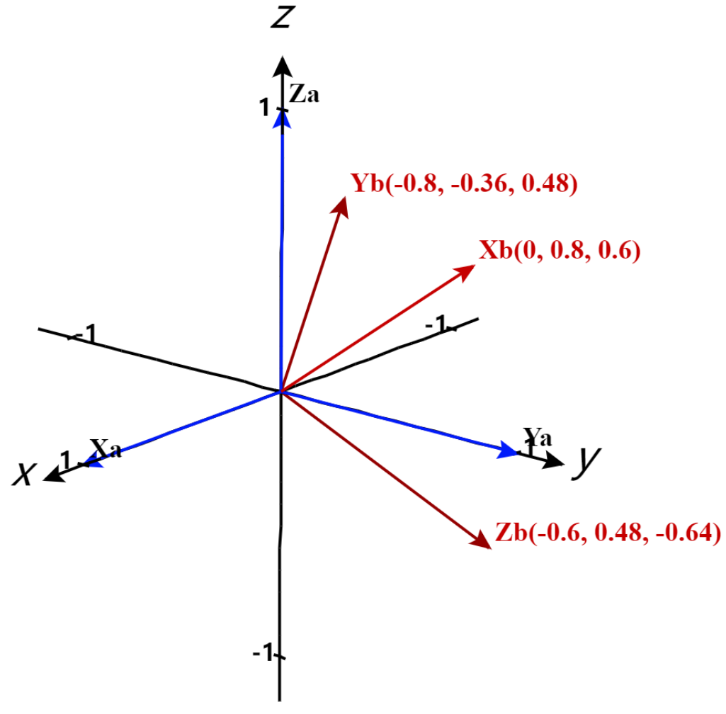
a来表示。之后对这个矩阵 $\mathbf E$ 应用一个旋转变换,以 $(0,-0.6,0.8)$ 为旋转轴,转90°。得到三个新的向量,用下标b来表示,记为 $\mathbf {X_b}= \left [ \begin{smallmatrix} 0 \\ 0.8 \\ 0.6 \end{smallmatrix} \right ] $ ,$\mathbf {Y_b} = \left [ \begin{smallmatrix} -0.8 \\ -0.36 \\ 0.48 \end{smallmatrix} \right ] $,$\mathbf {Z_b} = \left [ \begin{smallmatrix} -0.6 \\ 0.48 \\ -0.64 \end{smallmatrix} \right ] $ 根据基变换原理,易得旋转变换的矩阵表达式 $\mathbf R = \left [ \begin{smallmatrix} 0&-0.8 &-0.6 \\ 0.8&-0.36&0.48 \\ 0.6&0.48&-0.64 \end{smallmatrix} \right ]$ 计算得特征向量为 $(0,-0.75,1)$,发现这条向量即旋转轴!
此时我们考虑从 $\mathbf R$矩阵下变到 $\mathbf E$的变换矩阵是多少,即求 $\mathbf R$ 矩阵的逆
$$\mathbf R^{-1} = \left [ \begin{matrix} 0 & 0.8 & 0.6 \\-0.8 & -0.36 & 0.48 \\-0.6 & 0.48 & -0.64 \end{matrix}\right]$$观察形式大家就可以发现一个有趣的特点 $\mathbf R^{-1} = \mathbf R^T$
正交矩阵有一个几何直观的特点,表示一个旋转变换,并且矩阵的逆和矩阵的转置相等
根据特征值和特征向量这篇笔记中的内容,我们知道特征值是对一个变换(矩阵)特性的有力表征,公式 $\mathbf A \mathbf{\vec v} = \lambda \mathbf{\vec v}$ 表示了变换中被留在张成空间内的向量就是特征向量的符号表达,其中 $\vec v$ 是特征向量,$\lambda$ 即特征值
我们对上式进行一些数学恒等变换,左乘 $\vec v^T$,得到
$$\vec v^T \mathbf A \vec v = \vec v^T \lambda \vec v = \lambda \vec v^T \vec v \tag{2-1}$$此时我们会发现一些巧合,先来看看正定矩阵的正规定义:若一个 n×n的矩阵 $\mathbf M$ 是正定的,当且仅当队友所有的非零实系数的向量 $\vec v$,都有 $\vec v^T \mathbf M \vec v > 0$
我们暂时不考虑复数情况(在机器学习预见复数域的内容较少),结合上面的二公式,发现保证 $\vec v^T \mathbf M \vec v > 0$ 即使得 $\lambda \vec v^T \vec v>0$,其中 $\vec v^T \vec v$一定大于等于0(由于 $\vec v$ 是一个1×n的向量,转置进行矩阵相乘实际效果计算元素的平方和),所以可以推出即正定矩阵就是使得特征值大于0
再回到正定矩阵的定义公式 $\vec x^T \mathbf M \vec x > 0$,我们已经有深刻的理解 $\mathbf M \vec x$ 表示对向量 $\vec x$ 进行变换,记变换后的向量为 $\vec y = \mathbf M \vec x$ ,则我们可以把正定矩阵的公式写成
$$\vec x^T \vec y > 0 \tag{2-2}$$这个公式是不是很熟悉呢?它是两个向量的内积,对于内积,有公式:
$$\cos(\theta) = \frac{\vec x^T \vec y}{\Vert \vec x \Vert * \Vert \vec y \Vert} \hat {\jmath}$$$\Vert \vec x \Vert \; \Vert \vec y \Vert$ 表示 $\vec x$ 和 $\vec y$的长度,$\theta$ 是它们之间的夹角。根据2-2式,可以得到 $\cos(\theta) > 0$,即它们之间的夹角小于90度
总结:如果说一个矩阵正定,则表示,一个向量经过此矩阵变换后的向量与原向量夹角小于90度
当然,加一个【半】字,是指这个小于变成小于等于
矩阵中还有一张形状特殊的矩阵,被称为正规矩阵,定义为:如果矩阵 $\mathbf A$ 满足 $\mathbf A^T \mathbf A = \mathbf A \mathbf A^T$
更多的,如果矩阵 $\mathbf U$ 满足 $\mathbf U^T \mathbf U = \mathbf U \mathbf U^T = \mathbf I$,其中 $\mathbf I$ 是单位矩阵,则称矩阵 $\mathbf U$ 为酉矩阵
从变换的角度来看正规矩阵,先做一个变换 $\mathbf A$ 再做一个变换 $\mathbf A^T$。并且交换两个矩阵的位置,最终结果相同
在前面的三个描绘矩阵不同矩阵的概念中,多次使用了转置的概念。从矩阵形态的角度看,转置是将 $\mathbf A$ 的所有元素关于一条从第1行第1列元素出发的向右下方45度的射线作镜面翻转(下面的动图更加直观)
![]()
那么,从矩阵是表示变换的集合角度如何理解转置呢?
试图从另一个角度来理解其实也是为了回答另一个问题:为什么要定义转置这种操作呢?你可能会说,这就是一个【对角线镜像对称交换的操作】,从形式上来理解对一般人已完全足够。
这里要深究的原因也只是为了克服在学习机器学习的过程中,公式里若出现转置符号,无法完全理解带来的生涩感(俗称强迫症),对博主来说,一个直接动机源于SVD算法
首先,考虑矩阵的列向量有具体的列空间的含义(对应 $\hat {\imath}$ 和 $\hat {\jmath}$ 的变换位置),若进行转置操作,列空间的性质会被完全破坏,或者说,转换成了一个新的列空间
考虑矩阵转置的几何含义是无意义的,或者说,对出现过矩阵转置的公式的进一步理解是没有帮助的
特别的,如果是向量形式(1×n的矩阵),转置很多时候出现,是为了进行二次型运算(即平方运算),设 $\mathbf x = \{x_1, x_2,\ldots, x_n\}$ 是一个1×n的矩阵
很多机器学习的教材中这里会是列矩阵,因为要切合列空间的概念。对于机器学习来说,这里的 $x_1$ 代表的数据的特征维度
计算二次型: $\mathbf x \mathbf x^T = x_1^2 + x_2^2 + \ldots + x_n^2$ ,记过为一个数,表示的是距离
从列空间的概念,转置是一种非常特殊的旋转。这种旋转结合了横向镜面等特性,详细可以参看下图
从这幅图可以看出,如果想从几何变换的角度(类似3b1b的方法)来理解转置相当困难。此时,需要考虑换一种思考角度,性质和数学计算(这可能也是解决一个数学问题最常用的两种手段,性质寻找共性,并推广演绎,数学计算导出同样问题的不同表现形式,并总结规律)
首先先用一个简单的例子,二维可视化,并寻找规律,得到下面图像
![]()
观察得到,和旋转有一定的关系的,但是其实这个几何意义已经十分抽象了,为了追根之底,从数学的角度进行一些更有意思的探究
为了发掘 $\mathbf A$ 和 $\mathbf A^T$ 之间的关系,我们可以设有转换矩阵 $\mathbf T$,其描述了从 $\mathbf A$ 到 $\mathbf A^T$ 的变换,写成公式为:
$$
\mathbf T \mathbf A = \mathbf A^{T} \tag 1
$$
同时我们假设 $\mathbf A$ 是一个2×2的矩阵,如下所示所示(列的不同为字母的不同a和b,行的不同为小标的1和2)
保证变换不会压缩维度,即 $det(\mathbf A) \neq 0$,利用(1)式,未知数,消元计算后,可以算出 $\mathbf T$,其中 $det(\mathbf A) = a_1b_2 - b_1a_2$
$$\mathbf T = \frac{1}{det(\mathbf A)} \begin{bmatrix} a_{1} b_{2} - a_{2}^2 & a_{1} (a_{2} - b_{1}) \\ b_{2} (b_{1} - a_{2}) & a_{1} b_{2} - b_{1}^2 \\ \end{bmatrix} \tag{3}$$前面的 $\frac{1}{det(\mathbf A)}$ 作为一个常数,保证了 $det(\mathbf A^{T})=det(\mathbf A)$,将后面关键的变换矩阵写成
$$\mathbf T' = \begin{bmatrix} a_{1} b_{2} - a_{2}^2 & a_{1} (a_{2} - b_{1}) \\ b_{2} (b_{1} - a_{2}) & a_{1} b_{2} - b_{1}^2 \\ \end{bmatrix} \tag {4}$$把 (4)式进行整理,也写成矩阵相乘的形式,得到下式
$$\mathbf T'=\begin{bmatrix}\begin{bmatrix}a_{1} & a_{2} \\\end{bmatrix} \begin{bmatrix}b_{2} \\ -a_{2} \\\end{bmatrix} & \begin{bmatrix}a_{1} & a_{2} \\\end{bmatrix} \begin{bmatrix}-b_{1} \\ a_{1} \\\end{bmatrix} \\\begin{bmatrix}b_{1} & b_{2} \\\end{bmatrix} \begin{bmatrix}b_{2} \\ -a_{2} \\\end{bmatrix} & \begin{bmatrix}b_{1} & b_{2} \\\end{bmatrix} \begin{bmatrix}-b_{1} \\ a_{1} \\\end{bmatrix}\\\end{bmatrix} \tag{5}$$对于 $\mathbf A$ 的列空间来说,有 $\mathbf a = \left [ \begin{smallmatrix} a_1 \\ a_2 \end{smallmatrix} \right ]$ 和 $\mathbf b = \left [ \begin{smallmatrix} b_1 \\ b_2 \end{smallmatrix} \right ]$ 观察到 $\mathbf T$ 中包含列空间的两个项,把 $\mathbf T’$ 整理得
$$B'=\begin{bmatrix}{\mathbf a}^{T}\begin{bmatrix}b_{2} \\ -a_{2} \\\end{bmatrix} & {\mathbf a}^{T} \begin{bmatrix}-b_{1} \\ a_{1} \\\end{bmatrix} \\{\mathbf b}^{T} \begin{bmatrix}b_{2} \\ -a_{2} \\\end{bmatrix} & {\mathbf b}^{T} \begin{bmatrix}-b_{1} \\ a_{1} \\\end{bmatrix}\\\end{bmatrix}=\begin{bmatrix}{\mathbf a}\cdot\begin{bmatrix}b_{2} \\ -a_{2} \\\end{bmatrix} & {\mathbf a}\cdot \begin{bmatrix}-b_{1} \\ a_{1} \\\end{bmatrix} \\{\mathbf b}\cdot \begin{bmatrix}b_{2} \\ -a_{2} \\\end{bmatrix} & {\mathbf b}\cdot \begin{bmatrix}-b_{1} \\ a_{1} \\\end{bmatrix}\\\end{bmatrix} \tag{6}$$令 $\mathbf c = \begin{bmatrix}b_{2} \\ -a_{2} \\ \end{bmatrix} $ $\mathbf d = \begin{bmatrix}-b_{1} \\ a_{1} \\ \end{bmatrix} $ ,观察后发现规律:
$\mathbf c$ 和 $\mathbf d$ 组成的列空间设为 $\mathbf C$,写成公式为
$$\mathbf C = \begin{bmatrix}\mathbf c & \mathbf d\end{bmatrix} = \begin{bmatrix} b_2 & -b_1 \\ -a_2 & a_1\end{bmatrix} \tag{7}$$将(7)式左乘 $\mathbf A$ 得到下式
$$\mathbf A\mathbf C= \begin{bmatrix}a_{1} & b_{1} \\a_{2} & b_{2} \\\end{bmatrix}\cdot\begin{bmatrix}b_{2} & -b_{1} \\-a_{2} & a_{1} \\\end{bmatrix}=\begin{bmatrix}det(\mathbf A) & 0 \\0 & det(\mathbf A) \\\end{bmatrix} =det(\mathbf A) \mathbf I \tag{8}$$再将(8)式所有乘以 $\mathbf A$ 的逆矩阵 $\mathbf A^{-1}$ 得到
$$
\mathbf C = \mathbf A^{-1} det(\mathbf A) \tag{9}
$$
所以,构造的这个 $\mathbf C$ 矩阵和 $\mathbf A$ 矩阵的逆矩阵有关
另外,(4)式,即 $\mathbf T’$ 矩阵还可以被写成
$$\mathbf T'=\begin{bmatrix}\begin{bmatrix}\begin{bmatrix}a_{1} & b_{1} \\a_{2} & b_{2} \\\end{bmatrix}& \begin{bmatrix}b_{2} \\-a_{2} \\\end{bmatrix}\end{bmatrix}\\\begin{bmatrix}\begin{bmatrix}a_{1} & b_{1} \\a_{2} & b_{2} \\\end{bmatrix}& \begin{bmatrix}-b_{1} \\a_{1} \\\end{bmatrix}\end{bmatrix}\end{bmatrix}=\begin{bmatrix}\begin{bmatrix}\begin{bmatrix}a_{1} & b_{1} \\a_{2} & b_{2} \\\end{bmatrix}& \mathbf c\end{bmatrix}\\\begin{bmatrix}\begin{bmatrix}a_{1} & b_{1} \\a_{2} & b_{2} \\\end{bmatrix}& \mathbf d\end{bmatrix}\end{bmatrix} \tag{10}$$或者可以写成
$$\begin{align}\mathbf T' & = \begin{bmatrix}\begin{bmatrix}a_{1} & a_{2} \\\end{bmatrix} &\begin{bmatrix}b_{2} & -b_{1} \\-a_{2} & a_{1} \\\end{bmatrix} \\\begin{bmatrix}a_{2} & b_{2} \\\end{bmatrix}&\begin{bmatrix}b_{2} & -b_{1} \\-a_{2} & a_{1} \\\end{bmatrix}\\\end{bmatrix} = \begin{bmatrix}\mathbf a^{T}&\begin{bmatrix}\mathbf c & \mathbf d \\\end{bmatrix} \\\mathbf b^{T}&\begin{bmatrix}\mathbf c & \mathbf d \\\end{bmatrix}\\\end{bmatrix}\\ & = \begin{bmatrix}\mathbf c^{T}\mathbf C \\\mathbf d^{T}\mathbf C\\\end{bmatrix}=det(\mathbf A) \begin{bmatrix}\mathbf a^{T}\mathbf A^{-1}\\\mathbf b^{T}\mathbf A^{-1}\\\end{bmatrix} \end{align} \tag{11}$$由 $\mathbf T \mathbf A = \mathbf A^T$ 可得
$$\mathbf T= \begin{bmatrix} \mathbf a^T \mathbf A^{-1} \\ \mathbf b^T \mathbf A^{-1} \end{bmatrix} \tag{12}$$这时候,可以得出一个结论,矩阵的转置的过程和矩阵的逆是有关系的,是矩阵逆的一个更加复杂的表现形式
有了这个作为基础,考虑一下具有对称性,构造 $\mathbf A \mathbf A^T$,这个复合变换有着很好的对称性和分解性(接下来为了方便,默认非粗体表示的矩阵变换),因为
$$AA^T = \begin{bmatrix} a_1 & b_1 \\ a_2 & b_2\end{bmatrix}\begin{bmatrix} a_1 & a_2 \\ b_1 & b_2\end{bmatrix} = \begin{bmatrix} a_1^2 + b_1^2 & a_1a_2+b_1b_2 \\ a_1a_2+b_1b_2 & a_2^2 + b_2^2\end{bmatrix} \tag{13}$$考虑任何不进行压缩维度变换的矩阵都可以进行特征分解,则有
$$AA^{T} = R_{AA^{T}} \Lambda_{AA^{T}} (R^{-1})_{AA^{T}} \tag{14}$$之后左乘(这里补充一下,所有的左乘操作在几何意义上来说,就是附加了一个新的变换)$A^{-1}$,得到
$$A^{T} = A^{-1} R_{AA^{T}} \Lambda_{AA^{T}} (R^{-1})_{AA^{T}} \tag{15}$$根据之前(1)式的例子进行计算,发现 $R_{AA^{T}} = (R^{-1})_{AA^{T}}$,并且 $R_{AA^T}$ 首先将空间关于 y 轴对称,之后旋转 $\alpha$ 角度,所以假设定义
$$R_{AA^{T}}^{'} = \begin{bmatrix}cos \alpha & -sin \alpha \\sin \alpha & cos \alpha \\\end{bmatrix} \tag{16}$$利用上面的推导,带入(15)式,得到:
$$A^{T}=A^{-1} R_{AA^{T}}^{'} \begin{bmatrix}-1 & 0 \\0 & 1 \\\end{bmatrix}\Lambda_{AA^{T}} R_{AA^{T}}^{'}\begin{bmatrix}-1 & 0 \\0 & 1 \\\end{bmatrix} \tag{17}$$用更加清晰的符号改写(17)式得到
$$A^{T}=A^{-1} R_{\alpha} M_y \Lambda R_{\alpha} M_y \tag{18}$$$M_y$ 表示的是关于y轴对称
$R_\alpha$ 表示逆时针旋转 $\alpha$ 度
$\Lambda$ 表示一种伸缩变换
这里的(18式)结论和上面的作图规律,还有(12)式从某种程度上来说有相似的地方
其实应该从矩阵分解的部分来再次思索矩阵转置的意义,可详见什么是PCA,SVD
最终感觉关于转置还是研究的不够透彻,可能需要拔高到另一个层面去理解会更加直观,但是限于水平,只能至此(并不是数学专业的学生)