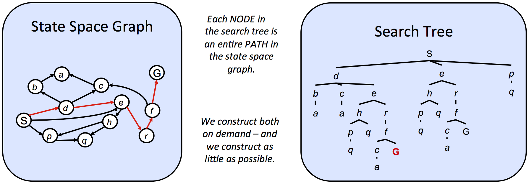
CS188 Search Lecture Notes III
Here are the notes for CS188 Local Search.
Local Search algorithms allow us to find local maxima or minima to find a configuration that satisfies some constraints or optimizes some objective function.
Hill-Climbing Search
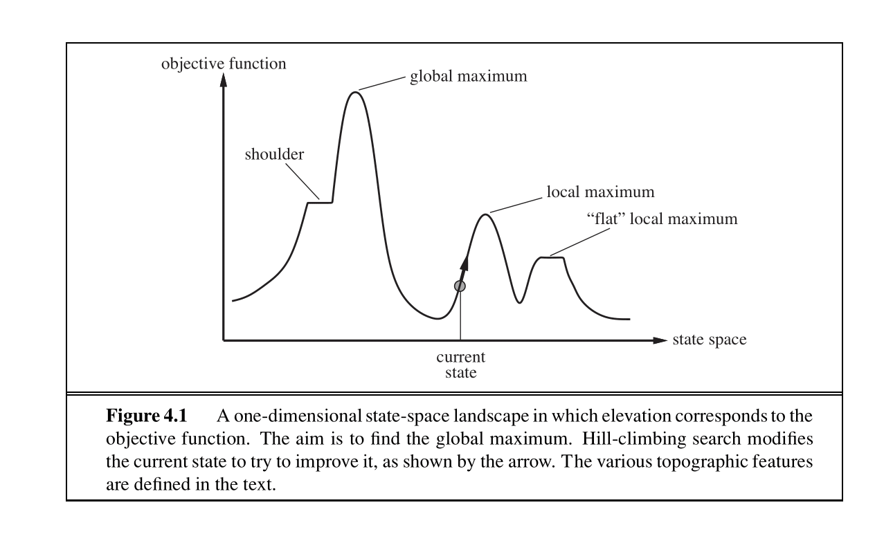
The hill-climbing search algorithm (or steepest-ascent) moves from the current state towards the neighboring state that increases the objective value the most.
The “greediness” of hill-climbing makes it vulnerable to being trapped in local maxima and plateaus.
There are variants of hill-climbing. The stochastic hill-climbing selects an action randomly among the possible uphill moves. Random sideways moves, allows moves that don’t strictly increase the objective, helping the algorithm escape “shoulders.”
1 | function HILL-CLIMBING(problem) returns a state |
The algorithm iteratively moves to a state with a higher objective value until no such progress is possible. Hill-climbing is incomplete.
Random-restart hill-climbing conducts a number of hill-climbing searches from randomly chosen initial states. It is trivially complete.
Simulated Annealing Search
Simulated annealing aims to combine random walk (randomly moving to nearby states) and hill-climbing to obtain a complete and efficient search algorithm.
The algorithm chooses a random move at each timestep. If the move leads to a higher objective value, it is always accepted. If it leads to a smaller objective value, the move is accepted with some probability.
This probability is determined by the temperature parameter, which initially is high (allowing more “bad” moves) and decreases according to some “schedule.”
Theoretically, if the temperature is decreased slowly enough, the simulated annealing algorithm will reach the global maximum with a probability approaching 1.
1 | function SIMULATED-ANNEALING(problem,schedule) returns a state |
Local Beam Search
Local beam search is another variant of the hill-climbing search algorithm.
The algorithm starts with a random initialization of states, and at each iteration, it selects new states. The algorithm selects the best successor states from the complete list of successor states from all the threads. If any of the threads find the optimal value, the algorithm stops.
The threads can share information between them, allowing “good” threads (for which objectives are high) to “attract” the other threads to that region as well.
1 | function LOCAL-BEAM-SEARCH(problem, k) returns a state |
Genetic Algorithms
Genetic Algorithms are a variant of local beam search.
Genetic algorithms begin as beam search with randomly initialized states called the population. States (called individuals) are represented as a string over a finite alphabet.
Their main advantage is the use of crossovers — large blocks of letters that have evolved and lead to high valuations can be combined with other such blocks to produce a solution with a high total score.
1 | function GENETIC-ALGORITHM(population, FITNESS-FN) returns an individual |
1 | function REPRODUCE(x, y) returns an individual |