defunbroadcast(grad, target_shape): # 如果形狀已經完美匹配,直接返回 if grad.shape == target_shape: return grad # 情況一:處理由於廣播而新增的前置維度(例如標量與矩陣運算) ndims_added = grad.ndim - len(target_shape) for _ inrange(ndims_added): grad = grad.sum(axis=0) # 情況二:處理被擴展的維度(原本大小為 1 的維度被擴展成了 N) for i, dim inenumerate(target_shape): if dim == 1: # 沿著被擴展的維度進行求和降維,並保持維度結構 grad = grad.sum(axis=i, keepdims=True) return grad
Natural Language Processing has undergone a massive evolution in recent years. To understand state-of-the-art models, we first need to look back at how we used to process sequences and the critical bottleneck that led to the invention of Attention.
The Foundation: Seq2Seq with RNNs
In traditional Sequence-to-Sequence (Seq2Seq) models—commonly used for tasks like machine translation—the architecture relies on Recurrent Neural Networks (RNNs) and consists of two main components:
Encoder RNN: Processes the input sequence x=(x1,x2,…,xT) and produces a sequence of hidden states h=(h1,h2,…,hT).
Decoder RNN: Generates the output sequence y=(y1,y2,…,yT′) step by step.
The encoder’s final hidden statehT is passed as the initial hidden state of the decoder. This vector—often called the context vector—carries a heavy burden: it must encode all necessary information from the entire input sequence.
The Context Bottleneck When dealing with long input sequences, a single fixed-size context vector struggles to capture all relevant details. Information inevitably gets lost or diluted, leading to poor model performance on longer text.
The Solution: The Attention Mechanism
To overcome the context bottleneck, the attention mechanism was introduced. It allows the decoder to dynamically focus on different parts of the input sequence at each decoding step, rather than relying on a single static vector.
How It Works Step-by-Step
At decoder timestep t, the model performs the following operations:
Compute Alignment Scores: Calculate the relevance between the current decoder state st−1 and each encoder hidden state hi:
eti=fattn(st−1,hi)
A common mathematical choice for this is:
eti=va⊤tanh(Wa[st−1;hi])
(Where Wa and va are learnable parameters, and [⋅;⋅] denotes concatenation). 2. Normalize Scores: Use a softmax function to convert the scores into probabilities (attention weights):
αti=∑j=1Texp(etj)exp(eti)
Compute the Context Vector: Create a weighted sum of the encoder hidden states using the attention weights:
ct=i=1∑Tαtihi
Decode: Use the new, time-dependent context vector ct in the decoder. This is typically done by concatenating ct with the decoder input yt−1, or feeding [ct;st−1] directly into the output layer to predict yt.
Key Advantages of Attention
Dynamic Focus: The model attends to the most relevant input tokens for each specific output step.
No Fixed Bottleneck: The full input sequence remains accessible throughout the entire decoding process.
Fully Differentiable: Attention weights are learned end-to-end via backpropagation, requiring no external supervision for alignment.
Generalizing to Attention Layers
In the Seq2Seq model, we can think of the decoder RNN states as Query Vectors and the encoder RNN states as Data Vectors. These get transformed to output Context Vectors. This specific operation is so powerful that it was extracted into a standalone, general-purpose neural network component: the Attention Layer.
To prevent vanishing gradients caused by large similarities saturating the softmax function, modern layers use Scaled Dot-Product Attention. Furthermore, separating the data into distinct “Keys” and “Values” increases flexibility, and processing multiple queries simultaneously maximizes parallelizability.
The Inputs
Query vectorQ [Dimensions: NQ×DQ]
Data vectorsX [Dimensions: NX×DX]
Key matrixWK [Dimensions: DX×DQ]
Value matrixWV [Dimensions: DX×DV]
(Note: The key weights, value weights, and attention weights are all learnable through backpropagation).
The Computation Process
Keys: The data vectors are projected into the key space.
K=XWK[NX×DQ]
Values: The data vectors are projected into the value space.
V=XWV[NX×DV]
Similarities: Calculate the dot product between queries and keys, scaled by the square root of the query dimension.
E=QKT/DQ[NQ×NX]
Eij=Qi⋅Kj/DQ
Attention Weights: Normalize the similarities using softmax along dimension 1.
A=softmax(E,dim=1)[NQ×NX]
Output Vector: Generate the final output as a weighted sum of the values.
Y=AV[NQ×DV]
Yi=j∑AijVj
Flavors of Attention
Depending on how we route the data, attention layers take on different properties:
Cross-Attention Layer: The data vectors and the query vectors come from two completely different sets of data.
Self-Attention Layer: The exact same set of vectors is used for both the data and the query. Because self-attention is permutation equivariant (it doesn’t inherently know the sequence order), we must add positional encoding to inject position information into each input vector.
Masked Self-Attention: We override certain similarities with negative infinity (−∞) before the softmax step. This strictly controls which inputs each vector is allowed to “look at” (often used to prevent looking into the future during text generation).
Multi-Headed Attention: We run H copies of Self-Attention in parallel, each with its own independent weights (called “heads”). We then stack the H independent outputs and use a final output projection matrix to fuse the data together.
The Rise of Transformers
Under the hood, self-attention boils down to four highly optimized matrix multiplications. However, calculating attention across every token pair requires O(N2) compute.
By taking these attention layers and building around them, we get the modern Transformer:
The Transformer Block A single block consists of a self-attention layer, a residual connection, Layer Normalization, several Multi-Layer Perceptrons (MLPs) applied independently to each output vector, followed by another residual connection and a final Layer Normalization.
Because they discard the sequential nature of RNNs, Transformers are incredibly parallelizable. Ultimately, a full Transformer Model is simply a stack of these identical, highly efficient blocks working together to process complex sequential data.
Applications
The true power of the Transformer lies in its versatility. By simply changing how data is pre-processed and fed into the model, the exact same attention mechanism can solve vastly different problems.
Large Language Models (LLMs)
Modern text-generation giants (like GPT-4 or Gemini) are primarily built on decoder-only Transformers. Here is how the pipeline flows:
Embedding: The model begins with an embedding matrix that converts discrete words (or sub-word tokens) into continuous, dense vectors.
Masked Self-Attention: These vectors are passed through stacked Transformer blocks. Crucially, these blocks use Masked Multi-Headed Self-Attention. The mask prevents the model from “cheating” by looking at future words, forcing it to learn sequence dependencies based only on past context.
Projection: After the final Transformer block, a learned projection matrix transforms each vector into a set of scores (logits) mapping to every word in the model’s vocabulary. A softmax function converts these into probabilities to predict the next word.
Vision Transformers (ViTs)
Who says Transformers are only for text? In 2020, researchers proved that the exact same architecture could achieve state-of-the-art results on images.
Patching: Instead of tokens, a ViT breaks an image down into a grid of fixed-size patches (e.g., 16x16 pixels).
Flattening: These 2D patches are flattened into 1D vectors and passed through a linear projection layer.
Positional Encoding: Because the model processes all patches simultaneously, positional encodings are added to retain the image’s 2D spatial relationships.
Unmasked Attention: Unlike LLMs, ViTs use an encoder-only architecture. There is no masking—the model is allowed to attend to the entire image at once to understand global context.
Pooling: At the end of the transformer blocks, the output vectors are pooled (or a special [CLS] classification token is used) to make a final prediction about the image.
Modern Architectural Upgrades
The original “vanilla” Transformer from the 2017 Attention is All You Need paper is rarely used exactly as written today. Researchers have introduced several key modifications to make models train faster, scale larger, and perform better.
Pre-Norm (vs. Post-Norm)
The original Transformer applied Layer Normalization after adding the residual connection (Post-Norm). Modern architectures apply it before the Attention and MLP blocks (Pre-Norm). This seemingly minor change drastically improves training stability, allowing researchers to train much deeper networks without the gradients blowing up or vanishing.
RMSNorm (Root Mean-Square Normalization)
Standard Layer Normalization is computationally expensive because it requires calculating the mean to center the data. RMSNorm is a leaner alternative that drops the mean-centering step entirely, scaling the activations purely by their Root Mean Square. This makes training slightly more stable and noticeably faster.
Given an input vector x of shape D, and a learned weight parameter γ of shape D, the output y is calculated as:
yi=RMS(x)xi∗γi
Where the Root Mean Square is defined as:
RMS(x)=ϵ+N1i=1∑Nxi2
(Note: ϵ is a very small number added to prevent division by zero).
SwiGLU Activation in MLPs
Inside a Transformer block, the output of the attention layer is passed through a Multi-Layer Perceptron (MLP). To understand the modern upgrade, let’s look at the classic setup versus the new standard.
The Classic MLP:
Input:X[N×D]
Weights:W1[D×4D] and W2[4D×D]
Output:Y=σ(XW1)W2[N×D]
Modern models (like LLaMA) have replaced this with the SwiGLU (Swish-Gated Linear Unit) architecture, which introduces a gating mechanism via element-wise multiplication (⊙):
The SwiGLU MLP:
Input:X[N×D]
Weights:W1 and W2[D×H], plus W3[H×D]
Output:Y=(σ(XW1)⊙XW2)W3
To ensure this new architecture doesn’t inflate the model’s size, researchers typically set the hidden dimension H=8D/3, which keeps the total parameter count identical to the classic MLP.
Interestingly, while SwiGLU consistently yields better performance and smoother optimization, the original authors famously quipped about its empirical nature in their paper:
“We offer no explanation as to why these architectures seem to work; we attribute their success, as all else, to divine benevolence.”
Mixture of Experts (MoE)
As models grow, compute costs skyrocket. MoE is a clever architectural trick to increase a model’s parameter count (its “knowledge”) without proportionately increasing the compute required to run it.
How it works: Instead of a single, massive MLP layer in each Transformer block, the model learns E separate, smaller sets of MLP weights. Each of these smaller MLPs is considered an “expert.”
Routing: When a token passes through the layer, a learned routing network decides which experts are best suited to process that specific token. Each token gets routed to a subset of the experts. These are the active experts.
The Benefit: This is called Sparse Activation. A 70-billion parameter MoE model might only activate 12 billion parameters per token. You get the capacity of a massive model with the speed and cost of a much smaller one.
Reference
Vaswani, A., Shazeer, N. M., Parmar, N., Uszkoreit, J., Jones, L., Gomez, A. N., Kaiser, L., & Polosukhin, I. (2017). Attention is All you Need. In Neural Information Processing Systems (pp. 5998–6008).
Recurrent Neural Networks (RNNs) are a class of neural networks designed to handle sequential data. Unlike standard feedforward networks, RNNs maintain an internal state (memory) that is updated as each element of a sequence is processed, allowing information to persist across time steps.
Sequence Architectures
RNNs are flexible and can be adapted to various input-output mapping structures depending on the task:
One-to-Many: A single input produces a sequence of outputs.
Example:Image Captioning (Input: Image → Output: Sequence of words).
Many-to-One: A sequence of inputs produces a single output.
Example:Action Prediction or Sentiment Analysis (Input: Sequence of video frames/words → Output: Label).
Many-to-Many: A sequence of inputs produces a sequence of outputs.
Example:Video Captioning (Input: Sequence of frames → Output: Sequence of words) or Video Classification (Frame-by-frame labeling).
The Recurrence Mechanism
The “key idea” behind an RNN is the use of a recurrence formula applied at every time step (t). This allows the network to process a sequence of vectors x by maintaining a hidden state h.
A. Hidden State Update
The hidden state is updated by combining the previous state with the current input.
ht=fW(ht−1,xt)
Parameters:
ht: New state (current hidden state).
ht−1: Old state (hidden state from the previous time step).
xt: Input vector at the current time step.
fW: A function (often a non-linear activation like tanh or ReLU) with trainable parameters W.
Note: the same function and the same set of parameters are used at every time step.
B. Output Generation
After the hidden state is updated, the network can produce an output at that specific time step.
yt=fWhy(ht)
Parameters:
yt: Output at time t.
ht: New state (the updated hidden state).
fWhy: A separate function with its own trainable parameters Why used to map the hidden state to the output space.
Backpropagation Through Time
Optimizing an RNN requires a specialized version of gradient descent known as Backpropagation Through Time (BPTT).
In its standard form, the model performs a complete forward pass through the entire sequence to calculate a global loss. During the subsequent backward pass, gradients are propagated from the final loss all the way back to the first time step.
While this captures long-range dependencies accurately, it is often computationally prohibitive for long sequences due to the massive memory requirements for storing intermediate states.
To mitigate these resource constraints, researchers often employ Truncated BPTT. This technique involves partitioning the sequence into smaller, manageable chunks.
The model performs a forward and backward pass on a specific chunk to update its weights before moving to the next. Crucially, while the hidden state is carried forward into the next chunk to maintain continuity, the gradient flow is “truncated” at the chunk boundary.
This approximation significantly reduces memory overhead and allows for the training of models on extended temporal data without sacrificing the benefits of sequential learning.
RNN Tradeoffs
RNNs can process input sequences of arbitrary length, and their model size remains constant regardless of input length since the same weights are shared across all time steps—ensuring temporal symmetry in how inputs are processed. In principle, they can leverage information from arbitrarily distant time steps.
However, in practice, recurrent computation tends to be slow due to its sequential nature, and capturing long-range dependencies remains challenging because relevant information from many steps back often becomes inaccessible or diluted over time.
Long Short Term Memory
Long Short Term Memory (LSTMs) are used to alleviate vanishing or exploding gradients when training long sequences by using a gated architecture that regulates the flow of information.
LSTM Mathematics
The operations of an LSTM cell at time step t are defined by three primary equations:
1. The Gate Vector LSTMs compute four internal vectors (gates and candidates) simultaneously by concatenating the previous hidden state ht−1 and the current input xt:
i (Input Gate): Decides which new information to store in the cell state.
f (Forget Gate): Decides which information to discard from the previous state.
o (Output Gate): Decides which part of the cell state to output.
g (Cell Candidate): Creates a vector of new candidate values (using tanh) to be added to the state.
2. The Cell State (ct) This is the “long-term memory” of the network. It is updated via a linear combination of the old state and the new candidates:
ct=f⊙ct−1+i⊙g
The use of the Hadamard product (⊙, element-wise multiplication) allows the forget gate to “zero out” specific memories while the input gate adds new ones. This additive update is the secret to preventing vanishing gradients.
3. The Hidden State (ht) The hidden state is the “working memory” passed to the next cell and the higher layers. It is a filtered version of the cell state:
Batch normalization and layer normalization improve training stability and reduce sensitivity to initialization by normalizing intermediate activations.
When training a deep neural network, the distribution of inputs to each layer can change as the network’s weights are updated. If the weights become too large, the inputs to subsequent layers may grow excessively; if the weights shrink toward zero, the inputs may diminish accordingly. These shifts in input distributions make training more difficult, as each layer must continuously adapt to changing conditions. This phenomenon is known as internal covariate shift.
Normalization allows us to use much higher learning rates and be less careful about initialization.
Plain Normalization
If normalization (e.g., centering the activations to zero mean) is performed outside of the gradient descent step, the optimizer will remain “blind” to the normalization’s effects.
In formal terms, if the optimizer treats the mean-subtraction operation as a fixed constant, the gradient updates will fail to reflect the true dynamics of the network.
Consider a layer that computes x=u+b and subsequently normalizes it: x^=x−E[x].
If the gradient ∂b∂ℓ is computed without considering how E[x] depends on b, the optimizer will attempt to adjust b to minimize the loss.
Because the normalization step subsequently subtracts the updated mean, the update Δb is effectively cancelled. The output x^ remains numerically identical to its state prior to the update:
(u+b+Δb)−E[u+b+Δb]=u+b−E[u+b]
Since the output—and consequently the loss—remains invariant despite the update, the optimizer will continue to increase b in a futile attempt to reach a lower loss. This results in unbounded parameter growth while the network’s predictive performance stagnates.
To maintain training stability, normalization must be included within the computational graph so that gradients correctly capture its dependence on the parameters.
However, performing full whitening across all examples can be computationally expensive. This is why techniques like Batch Normalization and Layer Normalization are used instead.
Batch Normalization
Batch Normalization performs normalization for each training mini-batch.
In Batch Normalization, we normalize each scalar feature independently, by making it have the mean of zero and the variance of 1.
x^(k)=Var[x(k)]+ϵx(k)−E[x(k)]
But simply normalizing each input of a layer may change what the layer can represent. The authors make sure that the transformation inserted in the network can represent the identity transform. Thus introducing:
y(k)=γ(k)x^(k)+β(k)
The parameters here are learnable along with the original model parameters, and restore the representation power of the network.
By setting γ(k)=Var[x(k)] and β(k)=E[x(k)], we could recover the original activations, if that were the optimal thing to do.
Algorithm 1: Batch Normalization Forward Pass
The forward pass of the Batch Normalization layer transforms a mini-batch of activations B={x1…m} into a normalized and linearly scaled output {yi}. This process ensures that the input to subsequent layers maintains a stable distribution throughout training.
Input: Values of x over a mini-batch: B={x1…m}; Parameters to be learned: γ,β. Output:{yi=BNγ,β(xi)}.
Mini-batch Mean:
μB←m1i=1∑mxi
Mini-batch Variance:
σB2←m1i=1∑m(xi−μB)2
Normalize:
x^i←σB2+ϵxi−μB
Scale and Shift:
yi←γx^i+β≡BNγ,β(xi)
Differentiation
To train the network using stochastic gradient descent, we must compute the gradient of the loss function ℓ with respect to the input xi and the learnable parameters γ and β. This is achieved by applying the chain rule through the computational graph of the BN transform.
1. Gradients for Learnable Parameters
The parameters γ and β are updated based on their contribution to all samples in the mini-batch:
Gradient w.r.t. β: Since ∂β∂yi=1, the gradient is the sum of the upstream gradients:
∂β∂ℓ=i=1∑m∂yi∂ℓ
Gradient w.r.t. γ: Since ∂γ∂yi=x^i, the gradient is the sum of the product of the upstream gradient and the normalized input:
∂γ∂ℓ=i=1∑m∂yi∂ℓ⋅x^i
2. Gradient w.r.t. Intermediate Statistics
The gradient propagates backward from yi to the normalized value x^i, and then to the batch statistics μB and σB2:
Gradient w.r.t. x^i:
∂x^i∂ℓ=∂yi∂ℓ⋅γ
Gradient w.r.t. σB2: This accounts for how the variance affects every x^i in the batch:
Finally, the gradient with respect to the original input xi is a combination of three paths: the direct path through x^i, the path through the variance σB2, and the path through the mean μB:
The normalization of activations allows efficient training, but is neither necessary nor desirable during inference. Thus, once the network has been trained, we use the normalization using the population, as opposed to the mini-batch:
x^=Var[x]+ϵx−E[x]
In practice, we use the fixed moving average calculated during training. During training, the mini-batch statistics are stochastic estimates of the true data distribution. The moving average serves as a stable, low-variance estimate of the population mean (E[x]) and population variance (Var[x]).
These running statistics are typically updated at each training step t using a momentum coefficient α (usually 0.9 or 0.99):
μ^new=αμ^old+(1−α)μB
σ^new2=ασ^old2+(1−α)σB2
Layer Normalization
Layer Normalization (LayerNorm) is an alternative normalization technique that normalizes across the features of a single sample rather than across a mini-batch.
For an input vector x∈Rd, LayerNorm computes the mean and variance over the feature dimension, ensuring that each individual sample has zero mean and unit variance.
Unlike Batch Normalization, it does not depend on batch statistics, which makes it particularly suitable for recurrent neural networks and transformer architectures where batch sizes may be small or variable.
Similar to BatchNorm, LayerNorm includes learnable parameters γ and β to scale and shift the normalized output, preserving the model’s representational capacity.
Reference
Ioffe, S., & Szegedy, C. (2015). Batch Normalization: Accelerating Deep Network Training by Reducing Internal Covariate Shift. arXiv:1502.03167.
Normalization layers standardize activations and then apply a learned scale and shift:
x^=σ2+ϵx−μ,y=γx^+β
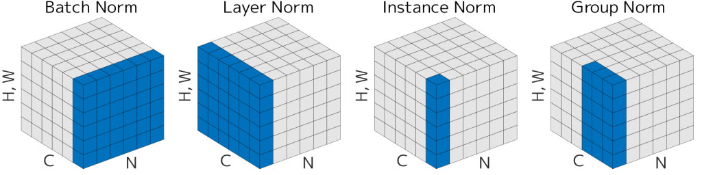
The difference between methods is which dimensions are used to compute μ and σ (for input shape N,C,H,W):
BatchNorm: per channel, over (N,H,W); depends on batch statistics
LayerNorm: per sample, over all features; independent of batch
InstanceNorm: per sample & channel, over (H,W); removes instance contrast
GroupNorm: per sample, over channel groups + spatial dims; stable for small batches
Key idea: same formula, different normalization axes → different behavior and use cases.
Regularization: Dropout
In each forward pass, randomly set a subset of activations to zero with probability p (a hyperparameter, often 0.5). To keep the expected activation unchanged, the remaining activations are scaled:
x~=1−pm⊙x,m∼Bernoulli(1−p)
This forces the network to have redundant representation, preventing co-adaptation of neurons
Acts like implicit ensemble averaging
Applied only during training; disabled at inference (no randomness)
With inverted dropout, no test-time scaling is needed because the activations were already rescaled during training.
Training: Add some kind of randomness
Testing: Average out randomness (sometimes approximate)
Activation Functions
Goal: Introduce non-linearity to the model.
Sigmoid:
Problem: the grandient gets small with many layers.
ReLU (Rectified Linear Unit):
Does not saturate
Converge faster than Sigmoid
Problem: not zero centered; dead when x<0.
GELU (Gaussian Error Linear Unit): f(x)=xΦ(x)
Smoothness facilitates training
Problem: higher computational cost; large negative values get small gradients
Case Study
AlexNet, VGG
Small filters, deep network.
The very first CNNs.
ResNet
Increasing the depth of a CNN does not always improve performance; in fact, very deep plain networks can exhibit the degradation problem, where training error increases as layers are added.
Although a deeper model should theoretically perform at least as well as a shallower one (since additional layers could learn identity mappings), in practice, standard layers struggle to approximate identity functions, making optimization difficult.
ResNet addresses this by reformulating the learning objective: instead of directly learning a mapping H(x), each block learns a residual function F(x)=H(x)−x, so the output becomes H(x)=F(x)+x.
The shortcut (skip) connection that adds the input x back to the learned residual improves gradient flow and makes it significantly easier to train very deep networks, especially when the desired transformation is close to identity.
Weight Initialization
If the value is too small, all activations tend to zero for deeper network layers.
for Din, Dout inzip(dims[:-1], dims[1:]): W = np.random.randn(Din, Dout) * np.sqrt(2 / Din) # Kaiming Initialization x = np.maximum(0, x.dot(W)) hs.append(x)
This makes the std almost constant. Activations are nicely scaled for all layers.
Data Preprocessing
Image Normalization: center and scale for each channel
Subtract per-channel mean and Divide by per-channel std (almost all modern models) (stats along each channel = 3 numbers)
Requires pre-computing means and std for each pixel channel (given your dataset)
Data Augmentation
We can do flips, random crops and scales, color jitters, random cutouts to enhance our training data.
Transfer Learning
How do we train without much data?
We can start with a large dataset like the ImageNet and train a deep CNN, learning general features.
With a small dataset, we can use the pretrained model and freeze most layers. We replace and reinitialize the final layer to match our new classes. We train only this last layer (a linear classifier).
With a bigger dataset, we can start from the pretrained model and initialize all layers with the pretrained weights. We then finetune more (or all) layers.
Deep learning frameworks provide pretrained models that we can transfer from:
A structured approach to stabilizing and optimizing deep learning training:
Step 1: Check Initial Loss
Verify the loss starts at a reasonable value (e.g., \log(\text{num_classes}) for classification). Large deviations typically indicate implementation issues such as incorrect labels or loss computation.
Step 2: Overfit a Small Sample
Train on a tiny subset (10–100 samples) and confirm the model can achieve near-zero loss. Failure here suggests problems with model capacity, optimization, or data preprocessing.
Step 3: Find a Working Learning Rate
Using the full dataset and a small weight decay (e.g., 10−4), test learning rates: 1e−1,1e−2,1e−3,1e−4,1e−5
Run ~100 iterations and select the rate that yields a clear, stable loss decrease.
Step 4: Coarse Hyperparameter Search
Explore a broad range of values (learning rate, weight decay, batch size, model size) using grid or random search. Train each configuration for ~1–5 epochs to identify promising regions.
Step 5: Refine the Search
Narrow the search around strong candidates and train longer. Optionally introduce schedules (e.g., cosine decay) or warmup.
Step 6: Analyze Curves
Inspect training vs. validation loss and accuracy:
Overfitting → increase regularization
Underfitting → increase capacity or training time
Instability → adjust learning rate or optimizer
Summary Insight
Most failures are due to basic setup issues (bad LR, incorrect loss, broken pipeline), not fine-grained hyperparameter choices. Systematic debugging is more effective than premature tuning.
When images get really large, we would have too many neurons to train in a regular neural network. The full connectivity is wasteful and the huge number of parameters would quickly lead to overfitting. What’s more, regular neural networks ignore the spatial structures of the image, missing out on some important information.
As a result, a new type of neural network, the Convolutional Neural Network (CNN) was developed.
Feature Extraction
Extract features from raw pixels to feed the model with more information.
Examples include Color Histogram and Histogram of Oriented Gradients. Hand-engineered features (e.g., HOG, SIFT) are largely obsolete in modern deep learning pipelines.
Stack them all together.
Traditional feature extraction is manually designed and fixed; CNNs learn hierarchical feature representations end-to-end.
Data and compute can solve problems better than human designers?
Linear Classification Intuition
Matrix multiplication involves vector dot products. Dot products measure how strongly an input aligns with learned feature directions, which act like soft, continuous templates.
Architecture
ConvNets use convolution and pooling operators to extract features while respecting 2D image structures.
The input remains a 3D tensor (e.g. 32x32x3), preserving spatial structures.
The layers of a ConvNet have neurons arranged in 3 dimensions: width, height, depth.
The neurons in a layer will only be connected to a small region of the layer before it.
We use three main types of layers to build ConvNet architectures: Convolutional Layer, Pooling Layer, and Fully-Connected Layer (exactly as seen in regular Neural Networks).
A simple ConvNet could have the architecture [INPUT - CONV - RELU - POOL - FC].
CONV layer will compute the output of neurons that are connected to local regions in the input, each computing a dot product between their weights and a small region they are connected to in the input volume.
POOL layer will perform a downsampling operation along the spatial dimensions (width, height).
ConvNets transform the original image layer by layer from the original pixel values to the final class scores.
The parameters in the CONV/FC layers will be trained with gradient descent.
Convolutional Layers
A convolutional layer performs a linear operation on the input using a set of learnable filters (also called kernels). Although commonly referred to as “convolution,” most deep learning libraries actually implement cross-correlation; the distinction is usually not important in practice.
The CONV layer’s parameters consist of a set of learnable filters. Each filter is spatially small but spans the full depth of the input.
Each filter typically has a single scalar bias, shared across all spatial positions in its activation map.
During the forward pass, each filter slides across the input volume. At every spatial location, the layer computes a dot product between the filter weights and the corresponding local region of the input, then adds a bias term. This produces a 2D activation map (feature map) for that filter.
A convolutional layer contains multiple filters. Each filter produces its own activation map, and these maps are stacked along the depth (channel) dimension to form the output volume. As a result, the number of filters determines the number of output channels.
Filters are initialized differently to break the symmetry.
For convolution with size K, each element in the output depend on a K×Kreceptive field. When you stack convolutional layers, the effective receptive field grows. Each deeper layer aggregates information from a larger region of the original input.
Apart from 2D conv, we also have 1D conv and 3D conv etc.
Zero Padding
Without zero-padding, feature maps may shrink with each layer. So we add padding around the input before sliding the filter.
With the input size W×W, filter size K×K, and padding size P, we get an output of size W−K+2×P.
A common setting is to set P as 2K−1, having the output of the same size of the input.
Stride
To increase effective receptive fields more quickly, we can skip some using strides.
With the input size W×W, filter size K×K, stride S, and padding size P, we get an output of size 2W−K+2×P+1.
In this way, we are downsampling the image and the receptive field grows exponentially.
Pooling
Pooling layers downsample a feature map by summarizing local neighborhoods.
In max pooling, a small window, such as 2×2, slides across the input and outputs the largest value in each window. This keeps the strongest local activation and reduces spatial resolution.
In average pooling, the layer outputs the mean value in each window instead of the maximum.
Translation Equivariance
CNNs use shared filters so the same local features can be detected at different positions in an image, while preserving information about where those features occur. This is called translation equivariance.
If you are diving into the mechanics of neural networks, you will inevitably encounter the backpropagation of the Softmax and Cross-Entropy loss. At first glance, the matrix calculus can feel a bit intimidating. However, once you break it down step-by-step using the chain rule, you will discover that the final gradients are incredibly elegant and intuitive.
In this post, we will walk through the complete mathematical derivation of the gradients for a linear classifier, moving from single variables to full matrix vectorization.
1. The Setup: Forward Propagation
Let’s define our variables for a single training sample. Assume our input features have a dimension of D, and we are classifying them into C distinct classes.
Input x: A D×1 column vector.
Weights W: A C×D matrix.
Bias b: A C×1 column vector.
True Label y: The true class index (or a C×1 one-hot encoded vector where only the true class index is 1).
The Linear Layer (Logits): First, we compute the raw scores (logits) z for each class:
z=Wx+b
The Softmax Layer: We convert these raw scores into a valid probability distribution. The probability of the sample belonging to class i is:
pi=∑j=1Cezjezi
The Cross-Entropy Loss: For a single sample where the true class is y, the loss only cares about the predicted probability assigned to that true class:
L=−log(py)
By substituting the Softmax formula into the loss function, we get:
L=−zy+log(j=1∑Cezj)
2. The Core Derivation: Gradient with respect to Logits (z)
To perform backpropagation, we first need to find how the loss changes with respect to each logit zi. We denote this gradient as ∂zi∂L.
We must split this into two scenarios: when i is the true class, and when i is any other class.
Case 1: Deriving for the true class (i=y)
∂zy∂L=∂zy∂(−zy+log(j=1∑Cezj))
Applying the chain rule to the logarithm term:
∂zy∂L=−1+∑j=1Cezj1⋅ezy
Notice that the fractional term is exactly our definition of py!
∂zy∂L=py−1
Case 2: Deriving for an incorrect class (i=y) Because zy does not contain zi, the derivative of the first term is 0.
∂zi∂L=0+∑j=1Cezj1⋅ezi
Again, the fractional term is pi:
∂zi∂L=pi
The Vectorized Form: We can beautifully combine these two cases using an indicator function I(i=y) (which is 1 if i is the true class, and 0 otherwise).
Let dz be the gradient vector ∂z∂L. Its vectorized form is simply:
dz=p−y
Intuition Check: This result is incredibly logical. The gradient is simply the Predicted Probability minus the True Probability. If the model is 100% confident and correct (py≈1), the gradient is 0, and no weights will be updated. The larger the error, the larger the gradient pushing the model to learn.
3. Gradients with respect to Weights (W) and Bias (b)
Now that we have the gradient of the loss with respect to the logits (dz), we use the chain rule to pass this error signal back to our parameters W and b.
Deriving for W: Let’s look at a single weight element Wij. It only influences the loss through the specific logit zi.
∂Wij∂L=∂zi∂L⋅∂Wij∂zi
Since zi=∑Wikxk+bi, the local gradient ∂Wij∂zi is simply xj. Therefore:
∂Wij∂L=dzi⋅xj
To vectorize this back into a C×D matrix (the same shape as W), we take the outer product of the column vector dz and the row vector xT:
∂W∂L=dz⋅xT
Deriving for b: Since z=Wx+b, the local derivative ∂b∂z is 1. Thus, the error signal passes directly through:
∂b∂L=dz
4. Scaling up: The Mini-Batch Form
In real-world training, we process N samples at a time to stabilize gradients and utilize parallel computing.
X becomes a D×N matrix.
dZ=P−Y becomes a C×N matrix.
To find the average gradient across the entire batch, we perform a matrix multiplication and divide by N:
Batch Weight Gradient:
∂W∂L=N1dZ⋅XT
Batch Bias Gradient: Sum the errors across all N samples for each class, then average:
∂b∂L=N1i=1∑NdZ(i)
Summary
By systematically applying the chain rule, we transformed a seemingly complex matrix calculus problem into clean, highly efficient linear algebra operations. Understanding this dz=p−y dynamic is the fundamental key to grasping how classification networks “learn” from their mistakes.
The primary goal of backpropagation is to calculate the partial derivatives of the cost function C with respect to every weight W and bias b in the network.
1. Notation (Matrix Form)
To facilitate a clean derivation using matrix calculus, we adopt the following conventions:
al: Activation vector of the l-th layer (nl×1).
zl: Weighted input vector of the l-th layer (nl×1), where zl=Wlal−1+bl.
Wl: Weight matrix of the l-th layer (nl×nl−1).
bl: Bias vector of the l-th layer (nl×1).
δl: Error vector of the l-th layer, defined as δl≡∂zl∂C.
σ′(zl): The derivative of the activation function applied element-wise to zl.
2. Derivation of the Equations
BP1: Error at the Output Layer
Goal: δL=∇aLC⊙σ′(zL)
Derivation Steps:
Apply the Chain Rule: The error δL represents how the cost C changes with respect to the weighted input zL. Since C depends on zL through the activations aL:
δL=∂zL∂C=(∂zL∂aL)T∂aL∂C
Compute the Jacobian: Because ajL=σ(zjL) (each output depends only on its own input), the Jacobian matrix ∂zL∂aL is a diagonal matrix:
∂zL∂aL=diag(σ′(z1L),…,σ′(znL))
Result: Multiplying a diagonal matrix by a vector is equivalent to the Hadamard product:
δL=∇aLC⊙σ′(zL)
BP2: Propagating Error to Hidden Layers
Goal: δl=((Wl+1)Tδl+1)⊙σ′(zl)
Derivation Steps:
Link Consecutive Layers: We express the error at layer l in terms of the error at layer l+1 using the multivariate chain rule:
δl=∂zl∂C=(∂zl∂zl+1)T∂zl+1∂C=(∂zl∂zl+1)Tδl+1
Differentiate the Linear Transformation: Recall zl+1=Wl+1al+bl+1 and al=σ(zl). Applying the chain rule to find ∂zl∂zl+1:
∂zl∂zl+1=∂al∂zl+1⋅∂zl∂al=Wl+1⋅diag(σ′(zl))
Transpose and Simplify: Substitute back and use the property (AB)T=BTAT:
Final Form: Convert the diagonal matrix multiplication to a Hadamard product:
δl=((Wl+1)Tδl+1)⊙σ′(zl)
BP3: Gradient for Biases
Goal: ∂bl∂C=δl
Derivation Steps:
Chain Rule via Intermediate z:
∂bl∂C=(∂bl∂zl)T∂zl∂C
Compute Local Gradient: From zl=Wlal−1+bl, we see that bl is added directly to the weighted sum. Thus, ∂bl∂zl is the Identity matrix I.
Conclusion:
∂bl∂C=ITδl=δl
BP4: Gradient for Weights
Goal: ∂Wl∂C=δl(al−1)T
Derivation Steps:
Element-wise Approach: Consider a single weight wjkl connecting neuron k in layer l−1 to neuron j in layer l:
∂wjkl∂C=∂zjl∂C∂wjkl∂zjl=δjl∂wjkl∂zjl
Solve for Partial Derivative: Since zjl=∑mwjmlaml−1+bjl, the derivative with respect to wjkl is simply akl−1. Therefore, ∂wjkl∂C=δjlakl−1.
Vectorize as an Outer Product: The collection of all such derivatives δjlakl−1 for all j,k forms the Outer Product of the error vector δl and the input activation vector al−1:
The number of neurson in the hidden layers is often related to the capacity of information. More neurons, more capacity.
A regularizer keeps the network simple and prevents overfitting. Do not use size of neural network as a regularizer. Use stronger regularization instead.
Derivatives
f(x,y)=x+y→∂x∂f=1,∂y∂f=1
f(x,y)=max(x,y)→∂x∂f=1(x≥y),∂y∂f=1(y≥x)
f(x,y)=xy→∂x∂f=y,∂y∂f=x
The derivative on each variable tells you the sensitivity of the whole expression on its value.
add gate: gradient distributor
mul gate: “swap multiplier”
copy gate: gradient adder
max gate: gradient router
Backpropagation
The problem now is to calculate the gradients in order to learn the parameters.
Obviously we can’t simply derive it on paper, for it can be very tedious and not feasible for complex models.
Here’s the better idea: Computational graphs + Backpropagation.
FORWARD PASS Computes output z from inputs x, y [ Input x ] ---------------------\ \ \ v _____________ | | | Node f | -----------------> [ Output z ] |_____________| ^ / / [ Input y ] ---------------------/
Gate / Node / Function object: Actual PyTorch code
1 2 3 4 5 6 7 8 9 10 11 12
classMultiply(torch.autograd.Function): @staticmethod defforward(ctx, x, y): ctx.save_for_backward(x, y) # Need to cache some values for use in backward z = x * y return z @staticmethod defbackward(ctx, grad_z): # Upstream gradient (grad_z) x, y = ctx.saved_tensors grad_x = y * grad_z # dz/dx * dL/dz <-- Multiply upstream and local gradients grad_y = x * grad_z # dz/dy * dL/dz return grad_x, grad_y
Aside: Vector Derivatives
For vector derivatives:
Vector to Scalar
x∈RN,y∈R
The derivative is a gradient.
∂x∂y∈RN(∂x∂y)n=∂xn∂y
Vector to Vector
x∈RN,y∈RM
The derivative is a Jacobian Matrix.
∂x∂y∈RN×M(∂x∂y)n,m=∂xn∂ym
Aside: Jacobian Matrix
A Jacobian Matrix is the derivative for a function that maps a Vector to a Vector.
Definition
Let f:Rn→Rm be a function such that each of its first-order partial derivatives exists on Rn. This function takes a point x=(x1,…,xn)∈Rn as input and produces the vector f(x)=(f1(x),…,fm(x))∈Rm as output.
Then the Jacobian matrix of f, denoted Jf, is the m×n matrix whose (i,j) entry is ∂xj∂fi; explicitly:
With the score function and the loss function, now we focus on how we minimize the loss. Optimization is the process of finding the set of parameters W that minimize the loss function.
Strategy #1: A first very bad idea solution: Random search
Core idea: iterative refinement
Strategy #2: Follow the slope
In 1-dimension, the derivative of a function:
dxdf(x)=h→0limhf(x+h)−f(x)
In multiple dimensions, the gradient is the vector of (partial derivatives) along each dimension ∇WL.
The slope in any direction is the dot product of the direction with the gradient The direction of steepest descent is the negative gradient.
Numerical Gradient
We can get an approximate numerical gradient. It is often sufficient to use a very small value (such as 1e-5).
This is easy to write, but might be slow.
Analytic Gradient
We can also use calculus to get the exact value of gradients.
Practical considerations
Always use analytic gradient, but check implementation with numerical gradient. This is called a gradient check.
It often works better to compute the numeric gradient using the centered difference formula: [f(x+h)−f(x−h)]/2h.
But in large-scale applications, the training data can have on order of millions of examples. It seems wasteful to compute the full loss function over the entire training set in order to perform only a single parameter update.
Stochastic Gradient Descent (SGD)
A very common approach to addressing this challenge is to compute the gradient over batches of the training data, which is called the Mini-batch Gradient Descent.
The gradient from a mini-batch is a good approximation of the gradient of the full objective. Therefore, much faster convergence can be achieved in practice by evaluating the mini-batch gradients to perform more frequent parameter updates.
The extreme case of this is a setting where the mini-batch contains only a single example. This process is called Stochastic Gradient Descent (SGD).
The size of the mini-batch is a hyperparameter. It is usually based on memory constraints (if any), or set to some value, e.g. 32, 64 or 128. We use powers of 2 in practice because many vectorized operation implementations work faster when their inputs are sized in powers of 2.
Problems with SGD
Jittering
Local minima or saddle points
Gradients from mini-batches might be too noisy.
SGD + Momentum
Momentum is a method that helps accelerate SGD in the relevant direction and dampens oscillations.
ρ (rho): Momentum coefficient (friction), typically 0.9 or 0.99.
α (alpha): Learning rate.
∇f(x): Gradient.
Aside: Nesterov Momentum
Standard Momentum calculates the gradient first, and then add the previous velocity to it.
Unlike Standard Momentum, Nesterov Momentum adds the previous velocity to the parameter first, and then calculate the gradient with the updated parameters. It looks ahead, making it more stable.
vt+1=ρvt−α∇f(xt+ρvt)
xt+1=xt+vt+1
We can let x~t=xt+ρvt to make it look nicer. Rearrange:
vt+1=ρvt−α∇f(x~t)
x~t+1=x~t−ρvt+(1+ρ)vt+1
=x~t+vt+1+ρ(vt+1−vt)
“Look ahead” to the point where updating using velocity would take us; compute gradient there and mix it with velocity to get actual update direction
RMSProp
RMSProp (Root Mean Square Propagation) is an adaptive learning rate optimization algorithm designed to improve the performance and speed of training deep learning models.
It adds element-wise scaling of the gradient based on historical sums of squares in each dimension (with decay).
Mathematical Formulation:
Compute Gradient
gt=∇θ
Update Moving Average of Squared Gradients
E[g2]t=γE[g2]t−1+(1−γ)gt2
Update Parameters
θt+1=θt−E[g2]t+ϵη⊙gt
where:
Learning Rate (η): Controls the step size during parameter updates.
Decay Rate (γ): Determines how quickly the moving average of squared gradients decays.
Epsilon (ϵ): A small constant (e.g., 1e-8) added to the denominator to prevent division by zero and ensure numerical stability.
1 2 3 4 5 6 7
grad_squared = 0 whileTrue: dx = compute_gradient(x) # Update moving average of the squared gradients grad_squared = decay_rate * grad_squared + (1 - decay_rate) * dx * dx # Update weights x -= learning_rate * dx / (np.sqrt(grad_squared) + 1e-7)
However, since the first and second momenet estimates start at zero, the initial step might be gigantic. So we implement bias correction to prevent early-stage instability.
For Standard Adam, the regularization is done in x before gradent computation.
For AdamW (Weight Dacay), the regularization term is added to the final x after the moments.
Learning Rate Schedules
The learning rate is a hyperparameter. We may make it decay over time.
Reduce learning rate at a few fixedpoints.
Cosine decay
Linear decay
Inverse sqrt decay
etc.
Empirical rule of thumb: If you increase the batch size by N, also scale the initial learning rate by N.
Second-Order Optimization
We can use gradient and Hessian to form a quadratic approximation, then step to its minima.
Second-Order Taylor Series:
J(θ)≈J(θ0)+(θ−θ0)⊤∇θJ(θ0)+21(θ−θ0)⊤H(θ−θ0)
Solving for the critical point we obtain the Newton parameter update:
θ∗=θ0−H−1∇θJ(θ0)
This can be bad for deep learning, for the amount of computation required.
Quasi-Newton methods (BGFS)
L-BGFS (Limited Memory BGFS): Does not store the full inverse Hessian.
Aside: Hessian Matrices
The Hessian matrix (or simply the Hessian), denoted as H, represents the second-order partial derivatives of a function. While the gradient (∇) tells you the slope (direction of steepest descent), the Hessian tells you the curvature of the loss function surface.
It is a square matrix of second-order partial derivatives of a scalar-valued function, f:Rn→R. It describes the local curvature of a function of many variables.
With the disadvantages of the KNN algorithm, we need to come up with a more powerful approach. The new approach will have two major components: a score function that maps the raw data to class scores, and a loss function that quantifies the agreement between the predicted scores and the ground truth labels.
Score Function
The score function maps the pixel values of an image to confidence scores for each class.
As before, let’s assume a training dataset of images xi∈RD, each associated with a label yi. Here i=1…N and yi∈1…K.
That is, we have N examples (each with a dimensionality D) and K distinct categories.
We will define the score function f:RD↦RK that maps the raw image pixels to class scores.
Linear Classifier
We will start out with arguably the simplest possible function, a linear mapping.
f(xi,W,b)=Wxi+b
In the above equation, we are assuming that the image xi has all of its pixels flattened out to a single column vector of shape [D x 1]. The matrix W (of size [K x D]), and the vector b (of size [K x 1]) are the parameters of the function.
The parameters in W are often called the weights, and b is called the bias vector because it influences the output scores, but without interacting with the actual data xi.
The input data are given and fixed. The goal is to set W,b in such way that the computed scores match the ground truth labels across the whole training set.
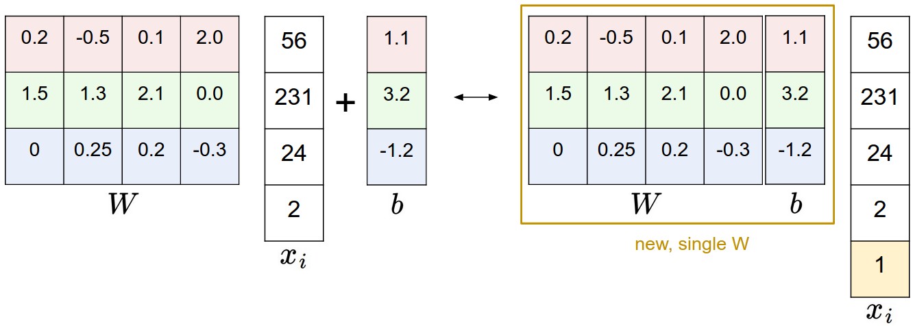
Bias Tricks
We can combine the two sets of parameters into a single matrix that holds both of them by extending the vector xi with one additional dimension that always holds the constant 1 - a default bias dimension.
f(xi,W)=Wxi
Image Data Preprocessing
In Machine Learning, it is a very common practice to always perform normalization of input features. In particular, it is important to center your data by subtracting the mean from every feature.
Loss Function
We will develop Multiclass Support Vector Machine (SVM) loss.
The score function takes the pixels and computes the vector f(xi,W) of class scores, which we will abbreviate to s (short for scores).
The Multiclass SVM loss for the i-th example is then formalized as follows:
Li=j=yi∑max(0,sj−syi+Δ)
The function accumulates the error of incorrect classes within Delta.
In summary, the SVM loss function wants the score of the correct class yi to be larger than the incorrect class scores by at least by Δ (delta).
The threshold at zero max(0, -) function is often called the hinge loss. We also have squared hinge loss SVM (or L2-SVM), which uses the form max(0, -)² that penalizes violated margins more strongly.
Regularization
We wish to encode some preference for a certain set of weights W over others to remove this ambiguity. We can do so by extending the loss function with a regularization penalty R(W). The most common regularization penalty is the squared L2 norm that discourages large weights through an elementwise quadratic penalty over all parameters:
R(W)=k∑l∑Wk,l2
Including the regularization penalty completes the full Multiclass Support Vector Machine loss, which is made up of two components: the data loss (which is the average loss Li over all examples) and the regularization loss.
Penalizing large weights tends to improve generalization, because it means that no input dimension can have a very large influence on the scores all by itself. It keeps the weights small and simple. This can improve the generalization performance of the classifiers on test images and lead to less overfitting.
It prevents the model from doing too well on the training data.
Note that due to the regularization penalty we can never achieve loss of exactly 0.0 on all examples.
Practical Considerations
Setting Delta: It turns out that this hyperparameter can safely be set to Δ=1.0 in all cases. (The exact value of the margin between the scores is in some sense meaningless because the weights can shrink or stretch the differences arbitrarily.)
Binary Support Vector Machine: The loss for the i-th example can be written as
Li=Cmax(0,1−yiwTxi)+R(W)
C in this formulation and λ in our formulation control the same tradeoff and are related through reciprocal relation C∝λ1.
Other Multiclass SVM formulations: Multiclass SVM presented in this section is one of few ways of formulating the SVM over multiple classes.
Another commonly used form is the One-Vs-All (OVA) SVM which trains an independent binary SVM for each class vs. all other classes. Related, but less common to see in practice is also the All-vs-All (AVA) strategy.
The last formulation you may see is a Structured SVM, which maximizes the margin between the score of the correct class and the score of the highest-scoring incorrect runner-up class.
Softmax Classifier
In the Softmax Classifier, we now interpret these scores as the unnormalized log probabilities for each class and replace the hinge loss with a cross-entropy loss that has the form:
where we are using the notation fj to mean the j-th element of the vector of class scores f.
The function fj(z)=∑kezkezj is called the softmax function: It takes a vector of arbitrary real-valued scores (in z) and squashes it to a vector of values between zero and one that sum to one.
Information Theory View
The cross-entropy between a “true” distribution p and an estimated distribution q is defined as:
H(p,q)=−x∑p(x)logq(x)
Minimizing Cross-Entropy is equivalent to minimizing the KL Divergence.
H(p,q)=H(p)+DKL(p∣∣q)
Because the true distribution p is fixed (its entropy H(p) is zero in this scenario), minimizing cross-entropy is the same as forcing the predicted distribution q to look exactly like the true distribution p.
The Softmax Loss objective is to force the neural network to output a probability distribution where the correct class has a probability very close to 1.0, and all other classes are close to 0.0.
Information Theory Supplementary
Information Entropy measures the uncertainty or unpredictability of a random variable.
The more unpredictable an event is (lower probability), the more information is gained when it occurs, and the higher the entropy. Conversely, if an event has a probability of 1 (certainty), its entropy is 0.
For a discrete random variable X with possible outcomes {x1,...,xn} and probabilities P(xi), the entropy H(X) is defined as:
H(X)=−i=1∑nP(xi)logP(xi)
Cross Entropy measures the total cost of using distribution q to represent distribution p.
Minimizing the cross-entropy H(p,q) is mathematically equivalent to minimizing the KL Divergence. It forces the predicted distribution q to become as close as possible to the true distribution p.
Probabilistic View
P(yi∣xi;W)=∑jefjefyi
The formula maps raw scores to a range of (0,1) such that the sum of all class probabilities equals 1.
Using the Cross-Entropy loss function during training is equivalent to maximizing the likelihood of the correct class.
Numeric Stability
Dividing large numbers can be numerically unstable, so it is important to use a normalization trick.
A common choice for C is to set logC=−maxjfj. This simply states that we should shift the values inside the vector f so that the highest value is zero. In code:
1 2 3 4 5 6
f = np.array([123, 456, 789]) # example with 3 classes and each having large scores p = np.exp(f) / np.sum(np.exp(f)) # Bad: Numeric problem, potential blowup
# instead: first shift the values of f so that the highest number is 0: f -= np.max(f) # f becomes [-666, -333, 0] p = np.exp(f) / np.sum(np.exp(f)) # safe to do, gives the correct answer
Note
To be precise, the SVM classifier uses the hinge loss, or also sometimes called the max-margin loss.
The Softmax classifier uses the cross-entropy loss.
SVM vs Softmax
The SVM interprets these as class scores and its loss function encourages the correct class to have a score higher by a margin than the other class scores.
The Softmax classifier instead interprets the scores as (unnormalized) log probabilities for each class and then encourages the (normalized) log probability of the correct class to be high (equivalently the negative of it to be low).
Softmax classifier provides “probabilities” for each class.
The “probabilities” are dependent on the regularization strength. They are better thought of as confidences where the ordering of the scores is interpretable.
In practice, SVM and Softmax are usually comparable. Compared to the Softmax classifier, the SVM is a more local objective.
The Softmax classifier is never fully happy with the scores it produces: the correct class could always have a higher probability and the incorrect classes always a lower probability and the loss would always get better.
However, the SVM is happy once the margins are satisfied and it does not micromanage the exact scores beyond this constraint.
Task: assigning an input image one label from a fixed set of categories
Images are defined as tensors of integers between [0,255], e.g. 800 x 600 x 3
Challenges:
Viewpoint variation
Scale variation
Deformation
Occlusion
Illumination conditions
Background clutter
Intra-class variation
A good image classification model must be invariant to the cross product of all these variations, while simultaneously retaining sensitivity to the inter-class variations.
The data-driven approach: first accumulating a training dataset of labeled images, then develop learning algorithms to learn about them.
The image classification pipeline:
Input: Input a set of N images, each labeled with one of K different classes.
Learn: use the training set to learn what every one of the classes looks like. training a classifier, or learning a model.
Evaluate: evaluate the quality of the classifier by asking it to predict labels for a new set of images that it has never seen before.
Nearest Neighbor Classifier
Here is the English translation of your content.
L1 Distance (Manhattan Distance)
L1 Distance is the sum of the absolute values of the differences between corresponding dimensions of two vectors. The calculation formula is:
L2 Distance is the square root of the sum of the squared differences between corresponding dimensions of two vectors. This is what we commonly refer to as the straight-line distance between two points. The calculation formula is:
Note on L2: Squaring amplifies values, thereby magnifying the influence of outliers.
Evaluation
For evaluation, we use accuracy, which measures the fraction of predictions that were correct.
k-Nearest Neighbr Classifier
The idea: we will find the top k closest images, and have them vote on the label of the test image.
Hyperparameters
It’s often not obvious what values/settings one should choose for hyperparameters.
We cannot use the test set for the purpose of tweaking hyperparameters.
-> Split your training set into training set and a validation set. Use validation set to tune all hyperparameters. At the end run a single time on the test set and report performance.
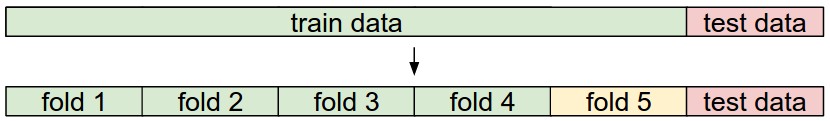
Cross-validation
Cross-validation: iterating over different validation sets and averaging the performance across these.
In this part of the Cache Lab, the mission is simple yet devious: optimize matrix transposition for three specific sizes: 32x32, 64x64, and 61x67. Our primary enemy? Cache misses.
Matrix Transposition
A standard transposition swaps rows and columns directly:
1 2 3 4 5 6 7 8 9 10 11 12
voidtrans(int M, int N, int A[N][M], int B[M][N]) { int i, j, tmp;
for (i = 0; i < N; i++) { for (j = 0; j < M; j++) { tmp = A[i][j]; B[j][i] = tmp; } }
}
While correct, this approach is a cache-miss nightmare because it ignores how data is actually stored in memory.
Cache Overview
To optimize effectively, we first have to understand our hardware constraints. The lab specifies a directly mapped cache with the following parameters:
Parameter
Value
Sets (S)
32
Block Size (B)
32 bytes
Associativity (E)
1 (Direct-mapped)
Integer Size
4 bytes
Capacity per line
8 integers
We will use Matrix Tiling and Loop Unrolling to optimize the codes.
32x32 Case
In this case, a row of the matrix needs 32/8 = 4 sets of cache to store. And cache conflicts occur every 32/4 = 8 rows. This makes 8x8 tiling the sweet spot.
By processing the matrix in 8×8 blocks, we ensure that once a line of A is loaded, we use all 8 integers before it gets evicted. We also use loop unrolling with 8 local variables to minimize the overhead of accessing B.
Since 61 and 67 are not powers of two, the conflict misses don’t occur in a regular pattern like they do in the square matrices. This “irregularity” is actually a blessing. We can get away with simple tiling. A 16x16 block size typically yields enough performance to pass the miss-count threshold.
1 2 3 4 5 6 7 8 9 10 11 12 13 14 15
int BLOCK_SIZE = 16; int i,j,k,l,tmp; int a,b; for(i = 0; i<N; i+=BLOCK_SIZE){ for(j = 0; j<M; j+=BLOCK_SIZE){ a = i+BLOCK_SIZE; b = j+BLOCK_SIZE; for(k = i; k<N && k<a; k++) { for(l = j; l<M && l<b; l++){ tmp = A[k][l]; B[l][k] = tmp; } } } }
64x64 Case
This is the hardest part. In a 64x64 matrix, a row needs 8 sets, but conflict misses occur every 32/8=4 rows. If we use 8x8 tiling, the bottom half of the block will evict the top half.
We can try a 4x4 matrix tiling first.
1 2 3 4 5 6 7 8 9 10 11 12 13 14 15
int BLOCK_SIZE = 4; int i,j,k,l,tmp; int a,b; for(i = 0; i<N; i+=BLOCK_SIZE){ for(j = 0; j<M; j+=BLOCK_SIZE){ a = i+BLOCK_SIZE; b = j+BLOCK_SIZE; for(k = i; k<N && k<a; k++) { for(l = j; l<M && l<b; l++){ tmp = A[k][l]; B[l][k] = tmp; } } } }
But this isn’t enough to pass the miss-count threshold.
We try a 8x8 matrix tiling. We solve this by partitioning the 8×8 block into four 4×4 sub-blocks and using the upper-right corner of B as a “buffer” to store data temporarily.
int i, j, k; int tmp1, tmp2, tmp3, tmp4, tmp5, tmp6, tmp7, tmp8;
// Iterate through the matrix in 8x8 blocks to improve spatial locality for (i = 0; i < N; i += 8) { for (j = 0; j < M; j += 8) { /** * STEP 1: Handle the top half of the 8x8 block (rows i to i+3) */ for (k = 0; k < 4; k++) { // Read 8 elements from row i+k of matrix A into registers tmp1 = A[i + k][j]; tmp2 = A[i + k][j + 1]; tmp3 = A[i + k][j + 2]; tmp4 = A[i + k][j + 3]; // Top-left 4x4 tmp5 = A[i + k][j + 4]; tmp6 = A[i + k][j + 5]; tmp7 = A[i + k][j + 6]; tmp8 = A[i + k][j + 7]; // Top-right 4x4
// Transpose top-left 4x4 from A directly into top-left of B B[j][i + k] = tmp1; B[j + 1][i + k] = tmp2; B[j + 2][i + k] = tmp3; B[j + 3][i + k] = tmp4;
// Temporarily store top-right 4x4 of A in the top-right of B // This avoids cache misses by using the already-loaded cache line in B B[j][i + k + 4] = tmp5; B[j + 1][i + k + 4] = tmp6; B[j + 2][i + k + 4] = tmp7; B[j + 3][i + k + 4] = tmp8; }
/** * STEP 2: Handle the bottom half and fix the temporary placement */ for (k = 0; k < 4; k++) { // Read bottom-left 4x4 column-wise from A tmp1 = A[i + 4][j + k]; tmp2 = A[i + 5][j + k]; tmp3 = A[i + 6][j + k]; tmp4 = A[i + 7][j + k]; // Read bottom-right 4x4 column-wise from A tmp5 = A[i + 4][j + k + 4]; tmp6 = A[i + 5][j + k + 4]; tmp7 = A[i + 6][j + k + 4]; tmp8 = A[i + 7][j + k + 4];
// Retrieve the top-right elements we temporarily stored in B in Step 1 int t1 = B[j + k][i + 4]; int t2 = B[j + k][i + 5]; int t3 = B[j + k][i + 6]; int t4 = B[j + k][i + 7];
// Move bottom-left of A into the top-right of B B[j + k][i + 4] = tmp1; B[j + k][i + 5] = tmp2; B[j + k][i + 6] = tmp3; B[j + k][i + 7] = tmp4;
// Move the retrieved temporary values into the bottom-left of B B[j + k + 4][i] = t1; B[j + k + 4][i + 1] = t2; B[j + k + 4][i + 2] = t3; B[j + k + 4][i + 3] = t4;
// Place bottom-right of A into the bottom-right of B B[j + k + 4][i + 4] = tmp5; B[j + k + 4][i + 5] = tmp6; B[j + k + 4][i + 6] = tmp7; B[j + k + 4][i + 7] = tmp8; } } }
Note: The key trick here is traversing B by columns where possible (so B stays right in the cache) and utilizing local registers (temporary variables) to bridge the gap between conflicting cache lines.
Conclusion
Optimizing matrix transposition is less about the math and more about mechanical sympathy—understanding the underlying hardware to write code that plays nice with the CPU’s cache.
The jump from the naive version to these optimized versions isn’t just a marginal gain; it’s often a 10x reduction in cache misses. It serves as a stark reminder that in systems programming, how you access your data is just as important as the algorithm itself.
A cache can be described with the following four parameters:
S=2s (Cache Sets): The cache is divided into sets.
E (Cache Lines per set): This is the “associativity.”
If E=1, it’s a direct-mapped cache. If E>1, it’s set-associative.
Each line contains a valid bit, a tag, and the actual data block.
B=2b (Block Size): The number of bytes stored in each line.
The b bits at the end of an address tell the cache the offset within that block.
m: The bits of the machine memory address.
2. Address Decomposition
When the CPU wants to access a 64-bit address, the cache doesn’t look at the whole number at once. It slices the address into three distinct fields:
Field
Purpose
Tag
Used to uniquely identify the memory block within a specific set. t = m - b - s
Set Index
Determines which set the address maps to.
Block Offset
Identifies the specific byte within the cache line.
3. The “Search and Match” Process
When our simulator receives an address (e.g., from an L or S operation in the trace file), it follows these steps:
Find the Set: Use the set index bits to jump to the correct set in our cache structure.
Search the Lines: Look through all the lines in that set.
Hit: If a line has valid == trueAND the tag matches the address tag.
Miss: If no line matches.
Handle the Miss:
Cold Start: If there is an empty line (valid == false), fill it with the new tag and set valid = true.
Eviction: If all lines are full, we must kick one out. This is where the LRU (Least Recently Used) policy comes in: we find the line that hasn’t been touched for the longest time and replace it.
Lab Requirements
For this Lab Project, we will write a cache simulator that takes a valgrind memory trace as an input.
Input
The input looks like:
1 2 3 4
I0400d7d4,8 M0421c7f0,4 L04f6b868,8 S7ff0005c8,8
Each line denotes one or two memory accesses. The format of each line is
1
[space]operation address,size
The operation field denotes the type of memory access:
“I” denotes an instruction load, “L” a data load,
“S” a data store
“M” a data modify (i.e., a data load followed by a data store).
Mind you: There is never a space before each “I”. There is always a space before each “M”, “L”, and “S”.
The address field specifies a 64-bit hexadecimal memory address. The size field specifies the number of bytes accessed by the operation.
CLI
Our program should take the following command line arguments:
getopt comes in unistd.h, but the compiler option is set to -std=c99, which hides all POSIX extensions. GNU systems provide a standalone <getopt.h> header. So we include getopt.h instead.
1
opt = getopt(argc, argv, "hvs:E:b:t:")
h and v: These are boolean flags.
s:, E:, b:, and t:: These are required arguments. The colon tells getopt that these flags must be followed by a value (e.g., -s 4).
After parsing the arguments, we set the initial value of our Cache Data Model.
fscanf does not skip spaces before %c, so we add a space before %c in the format string.
!feof(traceFile) does not work correctly here.It only returns true after a read operation has already attempted to go past the end of the file and failed. Using it as a loop condition (e.g., while (!feof(p))) causes an “off-by-one” error, where the loop executes one extra time with garbage data from the last successful read.
voidloadData(longlong address, int size) { // Simulate accessing data at the given address int s = getSetIndex(address); longlong t = getTag(address); global_timer++;
for (int i = 0; i < associativity; i++) { if (cache[s][i].valid && cache[s][i].tag == t) { hit_count++; cache[s][i].lru_counter = global_timer; if (verboseMode) printf(" hit"); return; } }
miss_count++; if (verboseMode) printf(" miss");
for (int i = 0; i < associativity; i++) { if (!cache[s][i].valid) { cache[s][i].valid = true; cache[s][i].tag = t; cache[s][i].lru_counter = global_timer; return; } }
eviction_count++; if (verboseMode) printf(" eviction");
int victim_index = 0; int min_lru = cache[s][0].lru_counter;
for (int i = 1; i < associativity; i++) { if (cache[s][i].lru_counter < min_lru) { min_lru = cache[s][i].lru_counter; victim_index = i; } }
We first check if the data already exists in the cache.
If it doesn’t exist, we have to scan for blank lines to load the data.
If blank lines don’t exist, we need to evict a line using the LRU strategy. We replace the victim line with the new line.
Other Operations
1 2 3 4 5 6 7 8 9 10 11
voidstoreData(longlong address, int size) { // Simulate storing data at the given address loadData(address, size); }
voidmodifyData(longlong address, int size) { // Simulate modifying data at the given address loadData(address, size); hit_count++; if (verboseMode) printf(" hit\n"); }
For this simulator, storing data and modifying data are basically the same thing as loading data.
Print Summary
We are asked to output the answer using the printSummary function.
In this project, we moved from the theory of hierarchy to the practical reality of memory management. By building this simulator, we reinforced several core concepts of computer systems.
With our simulator passing all the trace tests, we’ve effectively mirrored how a CPU “thinks” about memory. The next step is applying these insights to optimize actual code, ensuring our algorithms play nicely with the hardware we’ve just simulated.
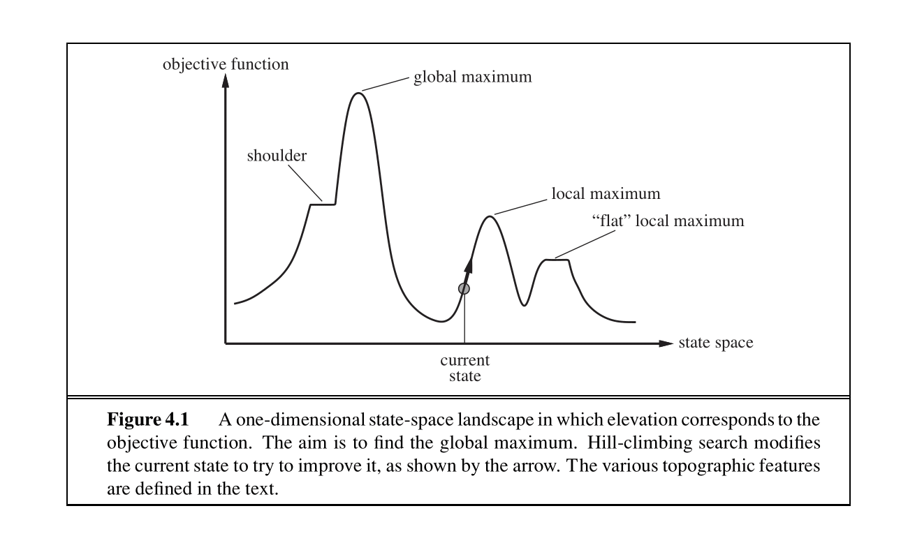
Local Search algorithms allow us to find local maxima or minima to find a configuration that satisfies some constraints or optimizes some objective function.
Hill-Climbing Search
The hill-climbing search algorithm (or steepest-ascent) moves from the current state towards the neighboring state that increases the objective value the most.
The “greediness” of hill-climbing makes it vulnerable to being trapped in local maxima and plateaus.
There are variants of hill-climbing. The stochastic hill-climbing selects an action randomly among the possible uphill moves. Random sideways moves, allows moves that don’t strictly increase the objective, helping the algorithm escape “shoulders.”
1 2 3 4 5 6 7
function HILL-CLIMBING(problem) returns a state current ← make-node(problem.initial-state) loop do neighbor ← a highest-valued successor of current if neighbor.value ≤ current.value then return current.state current ← neighbor
The algorithm iteratively moves to a state with a higher objective value until no such progress is possible. Hill-climbing is incomplete.
Random-restart hill-climbing conducts a number of hill-climbing searches from randomly chosen initial states. It is trivially complete.
Simulated Annealing Search
Simulated annealing aims to combine random walk (randomly moving to nearby states) and hill-climbing to obtain a complete and efficient search algorithm.
The algorithm chooses a random move at each timestep. If the move leads to a higher objective value, it is always accepted. If it leads to a smaller objective value, the move is accepted with some probability.
This probability is determined by the temperature parameter, which initially is high (allowing more “bad” moves) and decreases according to some “schedule.”
Theoretically, if the temperature is decreased slowly enough, the simulated annealing algorithm will reach the global maximum with a probability approaching 1.
1 2 3 4 5 6 7 8 9
function SIMULATED-ANNEALING(problem,schedule) returns a state current ← problem.initial-state for t = 1to ∞ do T ← schedule(t) if T = 0thenreturncurrent next ← a randomly selected successor ofcurrent ΔE ← next.value – current.value if ΔE > 0thencurrent ← next elsecurrent ← next onlywith probability e^(ΔE/T)
Local Beam Search
Local beam search is another variant of the hill-climbing search algorithm.
The algorithm starts with a random initialization of k states, and at each iteration, it selects k new states. The algorithm selects the k best successor states from the complete list of successor states from all the threads. If any of the threads find the optimal value, the algorithm stops.
The threads can share information between them, allowing “good” threads (for which objectives are high) to “attract” the other threads to that region as well.
1 2 3 4 5 6 7 8 9 10 11 12 13 14
function LOCAL-BEAM-SEARCH(problem, k) returns a state states ← k randomly generated states loop do if anystatein states is a goal then return that state all_successors ← an empty list for each statein states do all_successors.add( all successors of state ) current_best ← the highest valued statein all_successors if current_best.value ≤ max(states).value then return the highest valued statein states (Local Maxima Reached) states ← the k highest-valued states from all_successors
Genetic Algorithms
Genetic Algorithms are a variant of local beam search.
Genetic algorithms begin as beam search with k randomly initialized states called the population. States (called individuals) are represented as a string over a finite alphabet.
Their main advantage is the use of crossovers — large blocks of letters that have evolved and lead to high valuations can be combined with other such blocks to produce a solution with a high total score.
repeat new_population ← emptyset for i = 1to SIZE(population) do x ← RANDOM-SELECTION(population, FITNESS-FN) y ← RANDOM-SELECTION(population, FITNESS-FN) child ← REPRODUCE(x, y) if (small random probability) then child ← MUTATE(child) add child to new_population population ← new_population until some individual is fit enough, or enough time has elapsed returnthe best individual in population, according to FITNESS-FN
1 2 3 4 5
function REPRODUCE(x, y) returns an individual inputs: x, y, parent individuals
n ← LENGTH(x); c ← random number from 1 to n return APPEND(SUBSTRING(x, 1, c), SUBSTRING(y, c + 1, n))
Here are the lecture notes for UC Berkeley CS188 Lecture 3.
Heuristics
Heuristics are estimates of distance to goal states.
Heuristics are typically solutions to relaxed problems (where some of the constraints of the original problem have been removed).
With heuristics, it becomes very easy to implement logic in our agent that enables them to “prefer” expanding states that are estimated to be closer to goal states when deciding which action to perform.
Greedy Search
Greedy Search always selects the frontier node with the lowest heuristic value for expansion.
The frontier is represented by a priority queue.
Greedy search is not guaranteed to find a goal state if one exists, nor is it optimal. (If a very bad heuristic function is selected)
A* Search
A* search is a strategy for exploration that always selects the frontier node with the lowest estimated total cost for expansion.
A* search also uses a priority queue to represent its frontier.
A* search is both complete and optimal, if the heuristic is admissible.
g(n): The function representing total backwards cost computed by UCS.
h(n): The heuristic value function, or estimated forward cost, used by greedy search.
f(n): The function representing estimated total cost, used by A* search.
f(n)=g(n)+h(n)
Admissibility
The condition required for optimality when using A* tree search is known as admissibility.
Defining h∗(n) as the true optimal forward cost to reach a goal state from a given node n, we can formulate the admissibility constraint mathematically as follows:
∀n,0≤h(n)≤h∗(n)
Theorem. For a given search problem, if the admissibility constraint is satisfied by a heuristic function h, using A* tree search with h on that search problem will yield an optimal solution.
We can prove this theorem using proof by contradiction.
Graph Search
We keep track of which states you’ve already expanded, and never expand them again.
Tree search with this added optimization is known as graph search.
1 2 3 4 5 6 7 8 9 10 11
function A*-GRAPH-SEARCH(problem, frontier) return a solution or failure reached ← an empty dict mapping nodes to the costtoeach one frontier ← INSERT((MAKE-NODE(INITIAL-STATE[problem]),0), frontier) whilenotIS-EMPTY(frontier) do node, node.CostToNode ← POP(frontier) if problem.IS-GOAL(node.STATE) thenreturn node if node.STATE isnotin reached or reached[node.STATE] > node.CostToNode then reached[node.STATE] = node.CostToNode foreach child-node in EXPAND(problem, node) do frontier ← INSERT((child-node, child-node.COST + CostToNode), frontier) return failure
Note that in implementation, it’s critically important to store the reached set as a disjoint set and not a list.
Dominance
If heuristic a is dominant over heuristic b, then the estimated goal distance for a is greater than the estimated goal distance for b for every node in the state space graph. Mathematically,
∀n:ha(n)≥hb(n)
Dominance very intuitively captures the idea of one heuristic being better than another - if one admissible heuristic is dominant over another, it must be better because it will always more closely estimate the distance to a goal from any given state.
Additionally, the trivial heuristic is defined as h(n)=0, and using it reduces A* search to UCS.
All admissible heuristics dominate the trivial heuristic.
As a general rule, the max function applied to multiple admissible heuristics will also always be admissible.
Consistency
A heuristic function is said to be consistent, or monotone, if its estimate is always less than or equal to the estimated distance from any neighbouring vertex to the goal, plus the cost of reaching that neighbour.
Mathematically, this is expressed as the triangle inequality:
∀n,n′:h(n)≤c(n,n′)+h(n′)
where c(n,n′) is the actual cost of the edge from n to n′.
If h is consistent, the first time A* reaches a node, it is guaranteed to be via the optimal path.
Here are the lecture notes for UC Berkeley CS188 Lecture 1 and 2.
Agents
The central problem of AI is to create a rational agent. A rational agent is an entity that has goals or preferences and tries to perform a series of actions that yield the best/optimal expected outcome given these goals.
The agent exists in an environment. Together, the agent and the environment constitute the world.
Types of Agents
A reflex agent selects its action based on only the current state of the world.
A planning agent maintains a model of the world and uses this model to simulate performing various actions.
Sometimes agents fail due to wrong world models.
Task Environment
The PEAS (Performance Measure, Environment, Actuators, Sensors) description is used for defining the task environment.
The performance measure describes what utility the agent tries to increase.
The environment summarizes where the agent acts and what affects the agent.
The actuators and the sensors are the methods with which the agent acts on the environment and receives information from it.
Types of Environment
We can characterize the types of environments in the following ways:
partially observable environments
fully observable environments
Stochastic environments (uncertainty in the transition model)
deterministic environments
multi-agent environments
static environments
dynamic environments
environments with known physics
environments with unknown physics
State Space and Search Problems
A search problem consists of the following elements:
A state space - The set of all possible states that are possible in your given world
A set of actions available in each state
A transition model - Outputs the next state when a specific action is taken at current state
An action cost - Incurred when moving from one state to another after applying an action
A start state - The state in which an agent exists initially
A goal test - A function that takes a state as input, and determines whether it is a goal state
A search problem is solved by first considering the start state, then exploring the state space using the action and transition and cost methods, iteratively computing children of various states until we arrive at a goal state.
A world state contains all information about a given state, whereas a search state contains only the information about the world that’s necessary for planning.
State Space Graphs and Search Trees
A state space graph is constructed with states representing nodes, with directed edges existing from a state to its children. These edges represent actions, and any associated weights represent the cost of performing the corresponding action.
They can be noticeably large, but they represent states well. (All states occur only once)
Search trees encode the entire path (or plan) from the start state to the given state in the state space graph.
Since there often exist multiple ways to get from one state to another, states tend to show up multiple times in search trees.
Since these structures can be too large for computers, we can choose to store only states we’re immediately working with, and compute new ones on-demand.
Uninformed Search
The standard protocol for finding a plan from the start state to the goals is to maintain an outer frontier and continually expanding the frontier by replacing a node with its children.
Most implementations of such algorithms will encode information about the parent node, distance to node, and the state inside the node object. This procedure is known as tree search.
1 2 3 4 5 6 7 8
function TREE-SEARCH(problem, frontier) return a solution or failure frontier ← INSERT(MAKE-NODE(INITIAL-STATE[problem]), frontier) while not IS-EMPTY(frontier) do node← POP(frontier) if problem.IS-GOAL(node.STATE) then return node for each child-nodein EXPAND(problem, node) do add child-nodeto frontier return failure
The EXPAND function appearing in the pseudocode returns all the possible nodes that can be reached from a given node by considering all available actions.
When we have no knowledge of the location of goal states in our search tree, we are forced to do uninformed search.
The completeness of each search strategy - if there exists a solution to the search problem, is the strategy guaranteed to find it given infinite computational resources?
The optimality of each search strategy - is the strategy guaranteed to find the lowest cost path to a goal state?
The **branching factor ** - The increase in the number of nodes on the frontier each time a frontier node is dequeued and replaced with its children is . At depth k in the search tree, there exists nodes.
The maximum depth m.
The depth of the shallowest solution s.
Depth-First Search
Depth-First Search (DFS) always selects the deepest frontier node.
The frontier is represented by a stack.
Depth-first search is not complete. If there exist cycles in the state space graph, this inevitably means that the corresponding search tree will be infinite in depth.
Depth-first search is not optimal.
Breadth-Frist Search
Breadth-first search (BFS) always selects the shallowest frontier node.
The frontier is represented by a queue.
If a solution exists, then the depth of the shallowest node s must be finite, so BFS must eventually search this depth. Hence, it’s complete.
BFS is generally not optimal.
Iterative Deepening
Iterative Deepening (ID) is basically BFS implemented with DFS. It repeatedly executes depth-first search with an increasing depth limit.
The frontier is represented by a stack.
Iterative deepening is complete. Because it exhaustively searches each depth level before increasing the limit, it avoids the infinite loops of DFS and will find a solution if one exists at a finite depth.
ID is generally not optimal.
If the cost is uniform, ID and BFS will be optimal.
// edx = 14, esi = 0, edi = a intfunc4(int edi, int esi, int edx){ int mid = l + ((r-l)>>1); if(mid <= a){ if(mid==a){ return0; } l = mid + 1; return2*func4(a, l, r) + 1; }else{ r = mid - 1; return2*func4(a, l, r); } }
/* Hmm... Six phases must be more secure than one phase! */ input = read_line(); /* Get input */ phase_1(input); /* Run the phase */ phase_defused(); /* Drat! They figured it out! * Let me know how they did it. */ printf("Phase 1 defused. How about the next one?\n");
/* The second phase is harder. No one will ever figure out * how to defuse this... */ input = read_line(); phase_2(input); phase_defused(); printf("That's number 2. Keep going!\n");
/* I guess this is too easy so far. Some more complex code will * confuse people. */ input = read_line(); phase_3(input); phase_defused(); printf("Halfway there!\n");
/* Oh yeah? Well, how good is your math? Try on this saucy problem! */ input = read_line(); phase_4(input); phase_defused(); printf("So you got that one. Try this one.\n");
/* Round and 'round in memory we go, where we stop, the bomb blows! */ input = read_line(); phase_5(input); phase_defused(); printf("Good work! On to the next...\n");
/* This phase will never be used, since no one will get past the * earlier ones. But just in case, make this one extra hard. */ input = read_line(); phase_6(input); phase_defused();